Econometrics automation for Windows

eviews-mcp

Drive EViews 13 from Python — or let an AI assistant drive it for you. A Model Context Protocol server and a Python library, sharing one engine. Every number comes from EViews itself.

Created and maintained by Dr Merwan Roudane

PyPI v1.3.3 Licence MIT Python 3.10+ Platform Windows EViews 10–14 Tests 110 passing

$ pip install eviews-mcp

Read the researcher guide GitHub repository PyPI project

How it works

An AI assistant can write EViews code, but on its own it cannot run it — so it never learns whether the code worked, what the coefficients were, or which sample was used. It guesses, and guessed numbers are invented numbers.

With MCP in place the assistant runs the code, reads the real output, and continues from there. If the ADF test says p = 0.886, it sees 0.886.

The assistant cannot fabricate results, because the results come back from EViews. It can still misread them or choose a poor specification — you remain the econometrician — but the numbers are real.

Two ways to use it

As an MCP server

An assistant drives EViews conversationally. Best for exploration, diagnostics and getting unstuck.

Same engine

As a Python library

Write a script that drives EViews. Best for the final, reproducible version that ships with your paper.

Not a reimplementation

EViews does the maths

There is no second statistics engine here. Every coefficient on this page was computed by EViews.

Installation

Windows with a licensed EViews installation, and Python 3.10 or newer.

Install the package

:: with pandas support, recommended
pip install "eviews-mcp[pandas]"

This pulls mcp and pywin32 automatically.

Check EViews is reachable
```
python -c "from eviews_mcp import EViews; print(EViews().status())"
```
output verified on EViews 13.0
```
{'connected': True, 'progid': 'EViews.Manager', 'version': '13.0',
 'workfile': None, 'scratch_dir': 'C:\\ev_mcp'}
```
'connected': True is the thing to look for. EViews starts hidden if it was not already running — the first launch takes a few seconds.
You are ready

Use it as a library straight away, or connect an assistant below.

Connect an AI assistant

Any MCP-capable client works. Two of the most common:

Claude Code

One command

claude mcp add eviews -- eviews-mcp

Claude Desktop

Settings → Developer → Edit Config

{
  "mcpServers": {
    "eviews": {
      "command": "eviews-mcp"
    }
  }
}

Quit and reopen the application completely. The config file is only read at startup, so reloading the window is not enough. If eviews-mcp is not found, run where eviews-mcp and use the full path instead — remembering to double the backslashes inside JSON.

Confirm it worked by asking the assistant to “check the EViews connection”:

eviews_status real session output

Connected to EViews 13.0 via EViews.Manager
Scratch directory: C:\ev_mcp
Active workfile: none open (use create_workfile or open_workfile)

A complete study, end to end

A full ARDL exercise on 100 quarterly observations, exactly as it ran. The data were generated with a known long-run relationship — lngdp = 1.2 + 0.55·lnk + 0.35·lnl — so you can check the tool recovers it.

Load the data, then check what you actually loaded
“Import C:\ev_mcp\guide\macro.csv, then describe the workfile.”
import_data → workfile_info real session output
```
Imported C:\ev_mcp\guide\macro.csv.
Series now present: DATE, LNGDP, LNK, LNL

Workfile:       MACRO
Page:           Macro
Frequency:      Q
Page range:     1996Q1 2020Q4
Current sample: 1996Q1 2020Q4
Obs in range:   100
Obs in sample:  100
Objects:        4
```
EViews read the date column and structured the page itself. Confirming 100 observations takes five seconds and catches the worst class of silent error — see Traps.

Establish the order of integration

“Run an ADF test on lngdp in levels, then on the first difference.”

show("lngdp", "uroot") levels

Null Hypothesis: LNGDP has a unit root
Exogenous: Constant
Lag Length: 2 (Automatic - based on SIC, maxlag=12)

                                            t-Statistic  Prob.*

Augmented Dickey-Fuller test statistic      -0.500089    0.885575
Test critical values:   1% level            -3.49917
                        5% level            -2.89155
                        10% level           -2.58285

*MacKinnon (1996) one-sided p-values.

show("lngdp", "uroot(dif=1)") first difference

Null Hypothesis: D(LNGDP) has a unit root
Exogenous: Constant
Lag Length: 1 (Automatic - based on SIC, maxlag=11)

                                            t-Statistic  Prob.*

Augmented Dickey-Fuller test statistic      -12.1778     0.0001
Test critical values:   1% level            -3.49917
                        5% level            -2.89155
                        10% level           -2.58285

Unit root not rejected in levels (p = 0.886), strongly rejected in differences. lngdp is I(1), so the ARDL bounds framework applies.

Estimate the ARDL

equation ardl1.ardl(deplags=4, reglags=4) lngdp lnk lnl

show("ardl1") real session output

Dependent Variable: LNGDP
Method: ARDL
Sample: 1996Q2 2020Q4
Included observations: 99
Dependent lags: 4 (Automatic)
Automatic-lag linear regressors (4 max. lags): LNK LNL
Deterministics: Restricted constant and no trend (Case 2)
Model selection method: Akaike info criterion (AIC)
Number of models evaluated: 100
Selected model: ARDL(1,0,0)

Variable            Coefficient  Std. Error   t-Statistic  Prob.*

LNGDP(-1)           0.0155166    0.0978296    0.158608     0.874314
LNK                 0.53458      0.059789     8.94111      3.02733e-14
LNL                 0.365216     0.085789     4.25714      4.86164e-05
C                   1.13554      0.249799     4.54582      1.61133e-05

R-squared           0.985599     Mean dependent var        6.49484
Adjusted R-squared  0.985144     S.D. dependent var        0.239988
S.E. of regression  0.029251     Akaike info criterion     -4.18624
Sum squared resid   0.0812841    Schwarz criterion         -4.08139
Log likelihood      211.219      Hannan-Quinn criter.      -4.14382
F-statistic         2167.22      Durbin-Watson stat        2.02168
Prob(F-statistic)   2.60070e-87

Read the long-run relationship

“Show me the cointegrating relationship.”

show("ardl1", "cointrel") real session output

Deterministics: Rest. constant (Case 2)
------------------------------------------------------------
CE = LNGDP(-1) - (0.543006*LNK + 0.370972*LNL + 1.153436)
------------------------------------------------------------

    Variable *     Coefficient  Std. Error  t-Statistic  Prob.
------------------------------------------------------------
        LNK          0.543006    0.025016    21.70645    0.0000
        LNL          0.370972    0.080765     4.593229   0.0000
         C           1.153436    0.222325     5.188072   0.0000
------------------------------------------------------------
Note: * Coefficients derived from the CEC regression.

Estimated 0.543 and 0.371, against true values of 0.55 and 0.35. This view freezes into an EViews spool rather than a table, which cannot be read over COM at all — the package writes it out as text so you can see it.

Diagnose, then save

show("ardl1", "auto(2)") Breusch-Godfrey

Breusch-Godfrey Serial Correlation LM Test:
Null hypothesis: No serial correlation at up to 2 lags

F-statistic         1.47903      Prob. F(2,93)          0.233167
Obs*R-squared       3.05184      Prob. Chi-Square(2)    0.217421

No serial correlation (p = 0.233). Saving produces an ordinary .wf1 that opens in the EViews GUI like any other — nothing locks your work inside the tool.

Plots

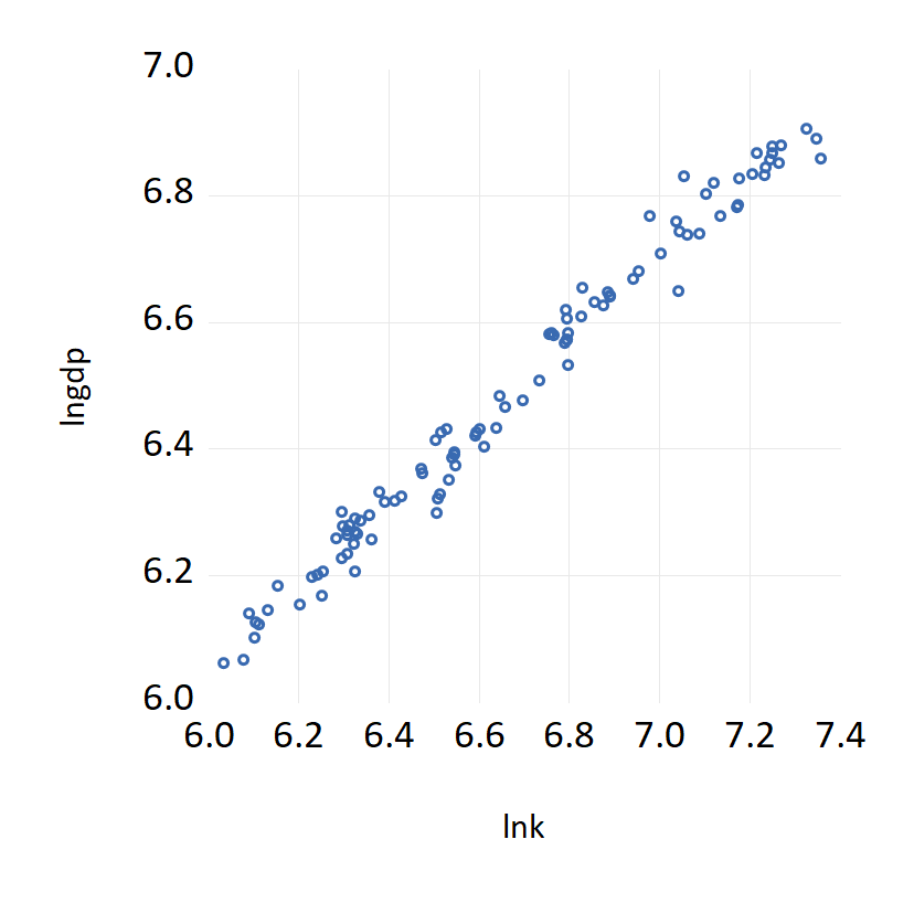
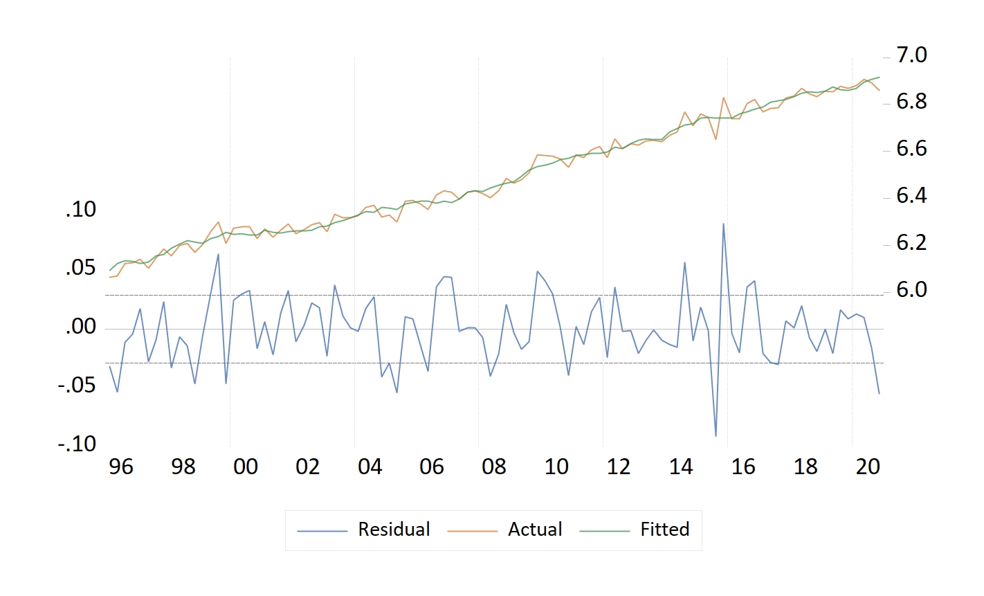
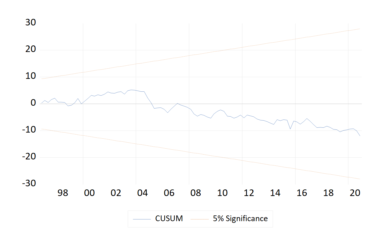
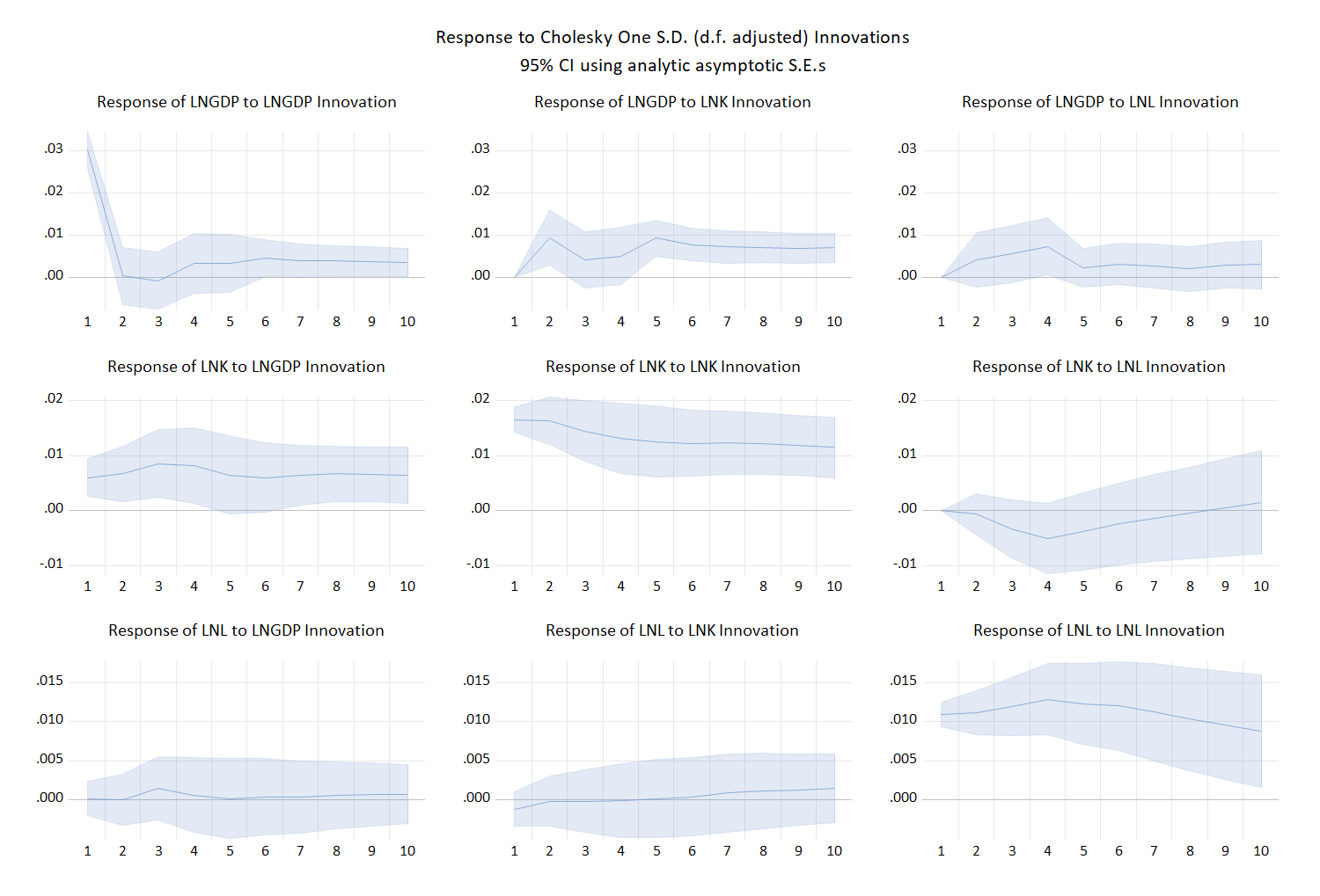
Graphs cannot be returned as text, so they are written to a file. Every image below was exported from the session above with a single call, at 200 dpi. Click any of them to open the full-resolution file.

Line chart of lngdp, lnk and lnl from 1996 to 2020, all trending upward. — **The three series**`export_object("g_series", "series-lines.png")`

Scatter plot of lngdp against lnk showing a tight positive linear relationship. — **Scatter, output against capital**`graph g_scat.scat lnk lngdp`

Actual, fitted and residual plot for the regression, residuals centred on zero. — **Actual, fitted, residual**`export_object("eq1", …, view="resids")`

CUSUM stability test plot with the statistic remaining inside the 5 percent bounds. — **CUSUM stability test**`view="rls(q)"`

Grid of impulse response functions from the three-variable VAR. — **VAR impulse responses**`view="impulse(10,m)"`

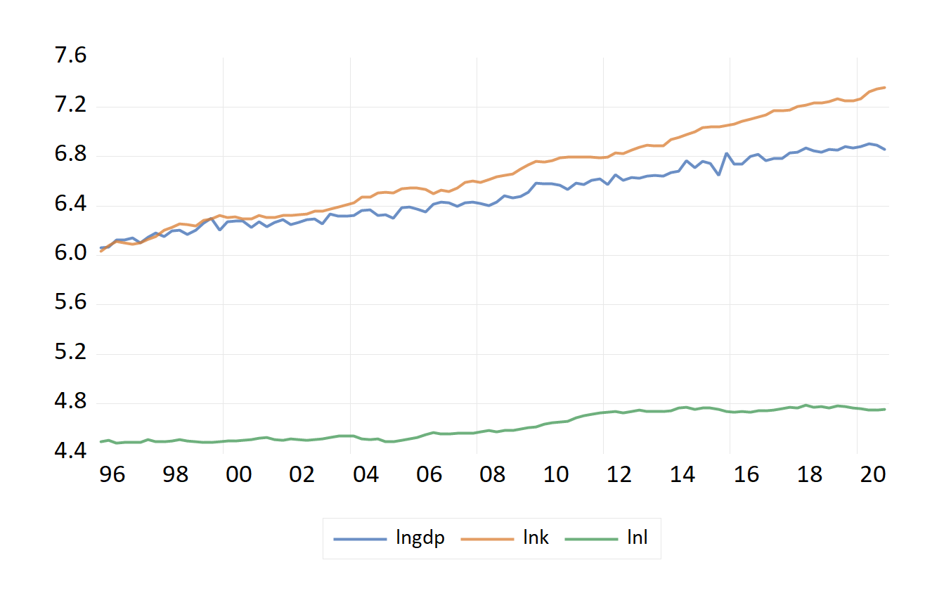
Not everything is a picture

A correlogram is a table, so it comes back as text rather than as a graph. The plotted autocorrelation bars are drawn by EViews and do not survive the trip across, but every number does.

show("lngdp", "correl") first 12 lags of 36

Sample: 1996Q1 2020Q4
Included observations: 100

Lag   AC           PAC          Q-Stat     Prob
1     0.957591     0.957591     94.4767    2.48e-22
2     0.925714     0.105209     183.669    1.31e-40
3     0.897812     0.047168     268.431    6.74e-58
4     0.868596     -0.016849    348.592    3.53e-74
5     0.840447     -0.00186816  424.432    1.6e-89
6     0.806486     -0.0839782   495.009    9.99e-104
7     0.778659     0.0404537    561.508    4.71e-117
8     0.750175     -0.015085    623.901    1.7e-129
9     0.723545     0.0144668    682.581    3.84e-141
10    0.694374     -0.0433673   737.225    6.37e-152
11    0.664384     -0.0258689   787.814    7.83e-162
12    0.633812     -0.040077    834.376    7e-171

Formats matter here. In raw EViews automation graph.save "figure.png" writes an EMF file with a .png name. This package derives the format from the extension and passes it explicitly, and a save that produces no file raises an error instead of reporting success. Graphs: png jpg pdf emf wmf bmp gif eps tex. Tables: csv rtf txt html.

Tool reference

The twenty-four tools an assistant has available. You never name them yourself — you ask in words — but knowing the vocabulary helps you ask precisely.

Tool	Purpose
Session
`eviews_status`	Connection, version and active workfile. Start here when debugging.
`reset_eviews`	Discard the instance and start a clean one.
`set_eviews_visible`	Show or hide the EViews window.
Workfiles
`create_workfile`	New page by frequency and range, e.g. quarterly 1990Q1–2020Q4.
`open_workfile`	Open an existing `.wf1` or `.wf2`.
`save_workfile`	Save, optionally to a new path.
`close_workfile`	Close one or all open workfiles. EViews caps how many may be open.
`workfile_info`	Name, page, frequency, range, sample and object count.
`list_objects`	Inventory, filterable by EViews type.
`set_sample`	Restrict the estimation sample.
Running code
`run_eviews_code`	Main tool. Runs a block of EViews program code — loops, conditionals, subroutines.
`run_program_file`	Run an existing `.prg`, with arguments.
`command`	A single command line.
Reading results
`show`	Renders any object or view as text. This is how results are read.
`evaluate`	One value from an expression, e.g. `eq1.@r2`.
`describe_object`	Object type, plus summary statistics for a series.
Analysis
`equation_coefficients`	Coefficients as a clean table of numbers, for reasoning about rather than reading.
`unit_root`	Tests the levels then successive differences, and reports the order of integration.
`diagnose_equation`	Breusch-Godfrey, White and Jarque-Bera in one call, each with its verdict.
Data
`read_data`	Series as an aligned table or full-precision CSV.
`write_series`	Write values from the conversation into a series.
`import_data`	Read `.xlsx`, `.csv`, `.dta`, `.sav` and more.
`export_data`	Write series to a file.
`export_object`	Save an object — the way to retrieve graphs.

Views: one object, many results

Every EViews view is reachable through show, so diagnostics need no special support. Ask in words — “test for heteroskedasticity” — and the assistant picks the view.

Ask for	View	What you get
Estimation output	default	The coefficient table
Unit root test	`uroot`	ADF on a series
Unit root on differences	`uroot(dif=1)`	ADF on Δx
Descriptive statistics	`stats`	Mean, SD, skew, Jarque-Bera
Correlogram	`correl`	ACF and PACF
Residual table	`resids(t)`	Actual, fitted, residual
Serial correlation	`auto(2)`	Breusch-Godfrey LM test
Heteroskedasticity	`white`	White test
Coefficient restriction	`wald c(2)=c(3)`	Wald test
Coefficient covariance	`coefcov`	Variance–covariance matrix
Long-run relation (ARDL)	`cointrel`	Cointegrating equation
Error-correction results	`ecresults`	ECM form
Granger causality (VAR)	`testexog`	Block exogeneity Wald tests
Impulse responses (VAR)	`impulse(t)`	IRF table
Variance decomposition	`decomp(10,t)`	Forecast error decomposition
Stability (CUSUM)	`rls(q)`	CUSUM test against 5% bounds
Recursive coefficients	`rls(c)`	Coefficient paths with plus/minus 2 S.E.

Some views draw rather than tabulate. resids and impulse are graphs by default; adding t — resids(t), impulse(t) — asks EViews for the table form instead.

The Python library

Conversation is good for finding a specification. It is poor for a paper, because a chat log is not a method section. The same work as a script:

from eviews_mcp import EViews

with EViews() as ev:
    ev.import_file(r"C:\data\macro.csv")

    # Order of integration
    for name in ("lngdp", "lnk", "lnl"):
        print(ev.show(name, "uroot"))
        print(ev.show(name, "uroot(dif=1)"))

    # Long-run model
    ev.run("equation ardl1.ardl(deplags=4, reglags=4) lngdp lnk lnl")
    print(ev.show("ardl1"))
    print(ev.show("ardl1", "cointrel"))
    print(ev.show("ardl1", "auto(2)"))

    print("R-squared:", ev.value("ardl1.@r2"))

    ev.export_object("ardl1", "residuals.png", view="resids")
    ev.save_workfile(r"C:\data\study.wf1")

Run it with python study.py and you get identical results on any machine with EViews. That file belongs in your replication package; the transcript does not.

pandas, in both directions

EViews → pandas

frame = ev.to_dataframe(
    ["lngdp", "lnk", "lnl"])
frame.describe()

Indexed by observation label — 1996Q1, 1996Q2, …

pandas → EViews

idx = pd.period_range(
    "2005Q1", periods=40, freq="Q")
df = pd.DataFrame({...}, index=idx)
ev.from_dataframe(df)

A dated index sets the page frequency and span, so dates stay aligned. Text columns are skipped.

Errors name the line

EViewsError passed through unchanged

BROKEN_COMMAND is not defined or is an illegal command in "BROKEN_COMMAND"
in MCP_77B699157F3B.PRG on line 2.

Traps that silently corrupt results

Properties of EViews automation that produce wrong numbers with no error message. The package defends against each one — worth knowing if you also write your own EViews scripts.

The trap	What this package does
Importing into an open workfile truncates your data. EViews cuts the file to the open page's length. A 100-row CSV read into a 12-row page becomes 12 rows, silently — every result afterwards computed on 12% of the data.	Imports create a new workfile sized to the file. Merging into the current page is opt-in.
The current sample governs writes, not just estimation. Under a restricted sample, writing 100 values writes only those inside it; the rest stay `NA`.	Writes default to the whole page.
A restricted sample persists until changed, so a later estimation silently uses it.	Every output header names the sample used. Read the `Sample:` line.
Graph exports ignore the file extension. `graph.save "figure.png"` writes an EMF file with a `.png` name.	Format derived from the extension and passed explicitly; a save producing no file raises.
Relative paths are not relative to you. EViews resolves them against its own working directory, so your file appears somewhere unrelated.	All paths are made absolute before being handed over.
EViews limits how many workfiles may be open, then refuses to create another.	`close_workfile` keeps long sessions healthy.

The five-second habit that catches most of these: read the four header lines on every EViews output — dependent variable, method, sample, included observations.

Author

Dr Merwan Roudane

Econometrician and package author. Creator of the QuantileOnQuantile, mqqr, qqkrls and mqqcause packages on CRAN, and of eviews-mcp.

GitHub profile Repository PyPI Report an issue

Citing this software

suggested wording methods or software note

Estimation was carried out in EViews 13, driven through the
eviews-mcp interface (Roudane, 2026).

Everything in one place

Resource	Link
PyPI package	pypi.org/project/eviews-mcp
Source code	github.com/merwanroudane/MCP_EVIEWS
Researcher guide	Zero to a finished ARDL study
Issue tracker	Report a bug or ask a question
Changelog	Release history
Install from	`pip install eviews-mcp`
Licence	MIT
Model Context Protocol	modelcontextprotocol.io
EViews	eviews.com