pragdml — Pragmatic DML with AI-learned representations

The problem it solves

You compress a rich covariate — a product description, an image, a clinical note — into an embedding, use it as a control, and report an ATE. That ATE is not the ATE you think it is.

Replacing the covariate $Z$ by a learned representation $X = x(Z,\lambda)$ changes two things at once: the regression you adjust with, and the population parameter your procedure is centred on. The paper's central identity says exactly how much.

\[\theta^{*} - \theta_{\lambda} \;=\; E\big[(g^{*}-g_{\lambda})(\alpha^{*}-\alpha_{\lambda})\big]\]

The gap is the product of two representation errors — one in the outcome regression $g$, one in the balancing weight (Riesz representer) $\alpha$. Not their sum.

Compress a lot, safely

The representation need not reconstruct $Z$. It only has to preserve one of the two objects. If either error is small, the target barely moves.

Fine-tune inside the folds

Learn the representation fold-wise and the usual DML inference still holds — with no stability or differentiability condition on the tuning algorithm.

When loss is material, get a region

An identified interval for the true parameter, root-$n$ inference for its endpoints, and a robustness value: one number for how strong the discarded information must be to overturn your sign.

Sixty seconds

import numpy as np
from pragdml import PragmaticDML

rng = np.random.default_rng(0)
X = rng.normal(size=(2000, 5))                 # your embedding goes here
e = 1 / (1 + np.exp(-X[:, 0]))                 # confounded assignment
D = (rng.uniform(size=2000) < e).astype(float)
Y = 2.0 * D + X[:, 0] - 0.5 * X[:, 1] + rng.normal(size=2000)

res = PragmaticDML(functional="ate", seed=0).fit(Y, D, X)
print(res.summary())
print("robustness value:", res.robustness_value())

                  Pragmatic DML -- ATE

  Observations      2000
  Folds (K)         5
  Variance          cross-fitted score variance (Eq. 12)
  Interval refers to: representation-based target (theta_lambda, Eq. 3)
==============================================================================
quantity estimate std_error       t p_value [95% CI lower  upper]
------------------------------------------------------------------------------
     ATE   2.0183    0.0479 42.1392  0.0000        1.9244  2.1122  ***
==============================================================================

Notice the line the table refuses to leave vague: which parameter the interval covers. That is the whole point of the method.

Theory

Setup

Observe $O=(Y,D,Z)$. Write $W^{*}=(D,Z)$ for the full information and $W_\lambda=(D,X)$ for what the representation retains. The targets are continuous linear functionals of the regression:

\[\theta^{*}=E[m(O,g^{*})],\qquad \theta_{\lambda}=E[m(O,g_{\lambda})].\]

For the binary ATE, $m(O,h)=h(1,Z)-h(0,Z)$, and $\theta_\lambda$ is the average predictive effect: the treatment contrast when you condition only on $(D,X)$.

The Riesz representer

Each functional has a unique $\alpha$ with $E[m(O,h)]=E[h\,\alpha]$. pragdml learns it variationally, by minimising the Riesz loss

\[L(\alpha)=E\big[\alpha(W)^2-2\,m(O,\alpha)\big],\]

which over the span of a feature map is a quadratic with a closed-form minimiser — the Riesz normal equations $Qc=r$, with $Q=P_n[\varphi\varphi']$ and $r_j=P_n[m(O,\varphi_j)]$. No propensity score is inverted, so no near-zero denominator can blow up.

The orthogonal score

\[\psi(O;g,\alpha)=m(O,g)+\alpha(W)\{Y-g(W)\}\]

Its population drift away from the target is exactly a mixed-bias term, $-E[(g-g_0)(\alpha-\alpha_0)]$, so first-stage error enters as a product rather than linearly. That is why each nuisance need only converge at $o(n^{-1/4})$, and why faster learning of one compensates for slower learning of the other.

The inferential hierarchy

You assume	The interval covers	At what variance
Assumption 1 only	$\theta_\lambda$, the representation's own target	the short score's
+ target adaptivity (Def. 1)	$\theta^{*}$, the causal parameter	the short score's
+ adaptive efficiency (Def. 2)	$\theta^{*}$	the semiparametric bound

Target adaptivity decides which parameter is covered; adaptive efficiency decides how wide the interval has to be. Every result object records which it is claiming.

Sensitivity, when adaptivity is not defensible

\[\theta^{*}-\theta_{0}=\rho\cdot C_Y\cdot C_D\cdot S\]

Term	Meaning	Identified?
$S^2=E[(Y-g_0)^2]\,E[\alpha_0^2]$	the scale of any possible bias	yes — estimated by DML
$C_Y^2$	share of residual outcome variation the omitted information could explain	no — you assume it
$C_D^2$	the same for the balancing weight	no — you assume it
$\rho\in[-1,1]$	alignment of the two omitted components	no — you assume it

$\rho$ is not a strength. Take $D=U^2$, $Y=D+U$. Here $U$ explains 100% of the residual variation in both equations — yet $U^2$ is uncorrelated with $U$, so the bias is exactly zero. Confounding must be strong and similarly shaped in both equations to bias anything.

Full step → equation map, including every proposition and both documented inconsistencies in the source paper →

API

Estimators

`PragmaticDML`	One information set. Cross-fitted DML with a learned Riesz representer (Theorem 1).
`PipelineDML`	A menu of pipelines, aggregated fold-wise on pooled out-of-fold predictions (Theorems 4–5).
`compare_information_sets`	The paper's Table 1: every information set side by side, plus the aggregate.
`pragmatic_dml`	One-call wrapper for users who never write classes.

Targets

`ATE`	$E[g(1,X)-g(0,X)]$ — binary treatment
`AverageDerivative`	$E[\partial_d g(d,X)\|_{d=D}]$ — continuous treatment (Eq. 67)
`ATT`	a ratio target, with a delta-method correction
`AveragePotentialOutcome`, `WeightedATE`, `PolicyEffect`	further members of the Riesz-linear class

Sensitivity

`res.sensitivity()`	the `SensitivityAnalysis` for a fit
`.interval(cy2=, cd2=, rho=)`	the identified region (Eq. 51)
`.evaluate(..., method=)`	endpoints, standard errors and a confidence envelope
`.grid(...)`	the Table 3 scenario layout
`.robustness_value()`	the breakdown strength
`benchmark_covariate(...)`	calibrate scenarios from observed covariates

Diagnostics

`omitted_information_gap`	Proposition 1, with the exact gap and its Cauchy–Schwarz bound
`target_adaptivity`, `adaptive_efficiency`	Definitions 1–2
`product_rate`, `pooling_conditions`	Eqs. (32), (45), (49) — evaluated on your numbers

Complete application: 401(k) and net financial assets

The package ships the 1991 SIPP extract — 9,915 households, the canonical dataset of this literature and the empirical application of the parent paper. Run it with python examples/pension_401k.py.

The question. 401(k) eligibility is not randomised: it depends on your employer. The naive gap in net financial assets is $19,559, and it is confounded. How much survives adjustment — and how strong would unobserved firm characteristics have to be to overturn what is left?

from pragdml import PragmaticDML
from pragdml.datasets import load_pension

Y, D, X = load_pension(return_X_y=True)
res = PragmaticDML(functional="ate", n_rep=5, seed=20261017).fit(Y, D, X)
sa  = res.sensitivity()

$19,559

naive gap

$7,855

adjusted ATE
se $1,392

4.2%

robustness value
published: 4.5%, 5.4%

The 95% interval [$5,126, $10,583] contains both figures the parent paper reports (about $9,000 and about $8,000), from a different nuisance learner.

How fragile is it?

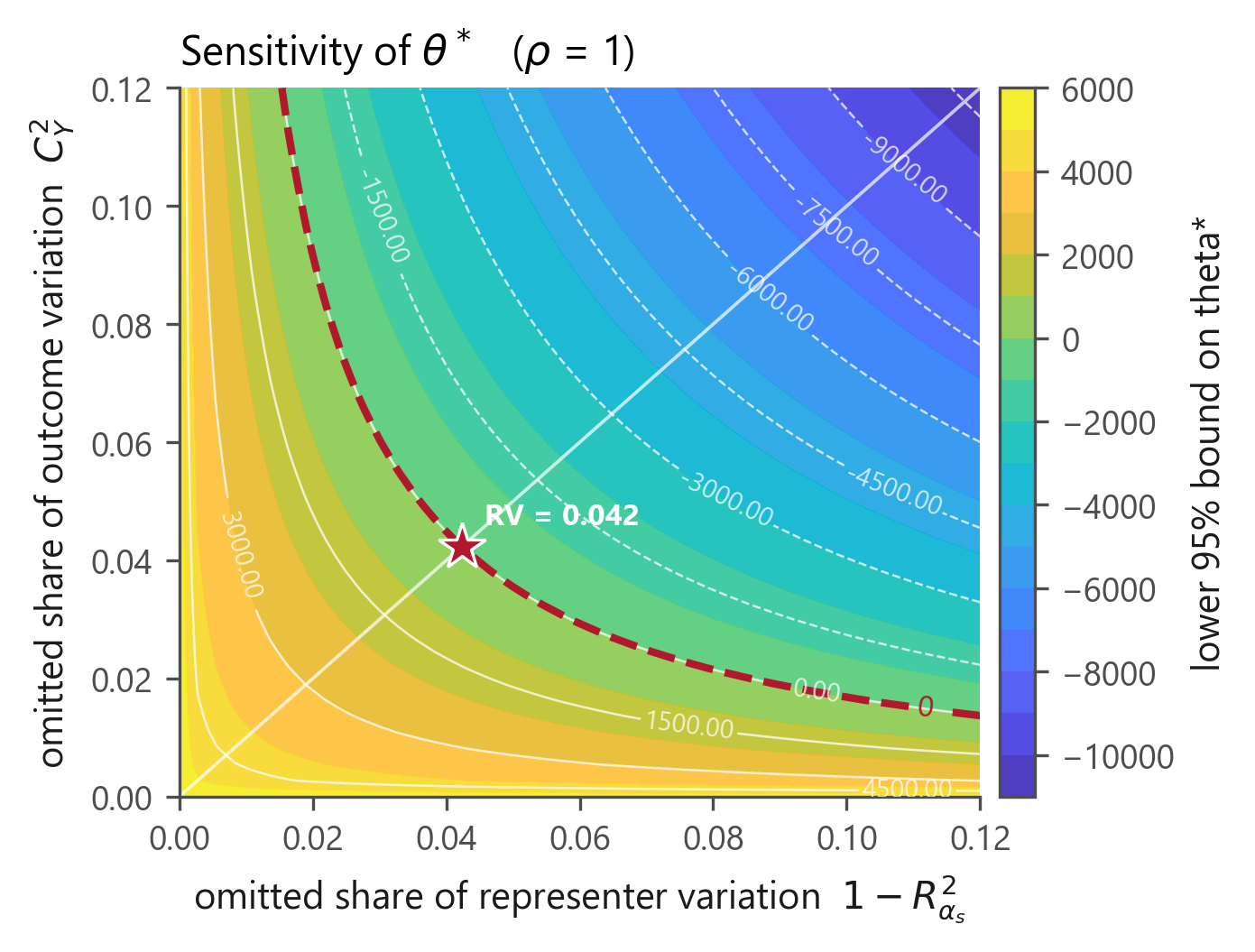
Sensitivity contour plot: lower 95% bound on the causal effect across confounding scenarios, with the zero contour and robustness value marked — Every point is a confounding scenario. Colour is the lower 95% bound on the true effect. The **red dashed line is where that bound hits zero**; beyond it the sign is no longer safe. The star sits where the 45° line crosses it — that is the robustness value, and it is why one number can stand in for the whole picture.

Reading it: unobserved firm characteristics explaining less than 4.2% of the residual variation — both of the outcome and of the treatment, in the worst-case alignment $\rho=1$ — cannot bring the lower confidence limit to zero.

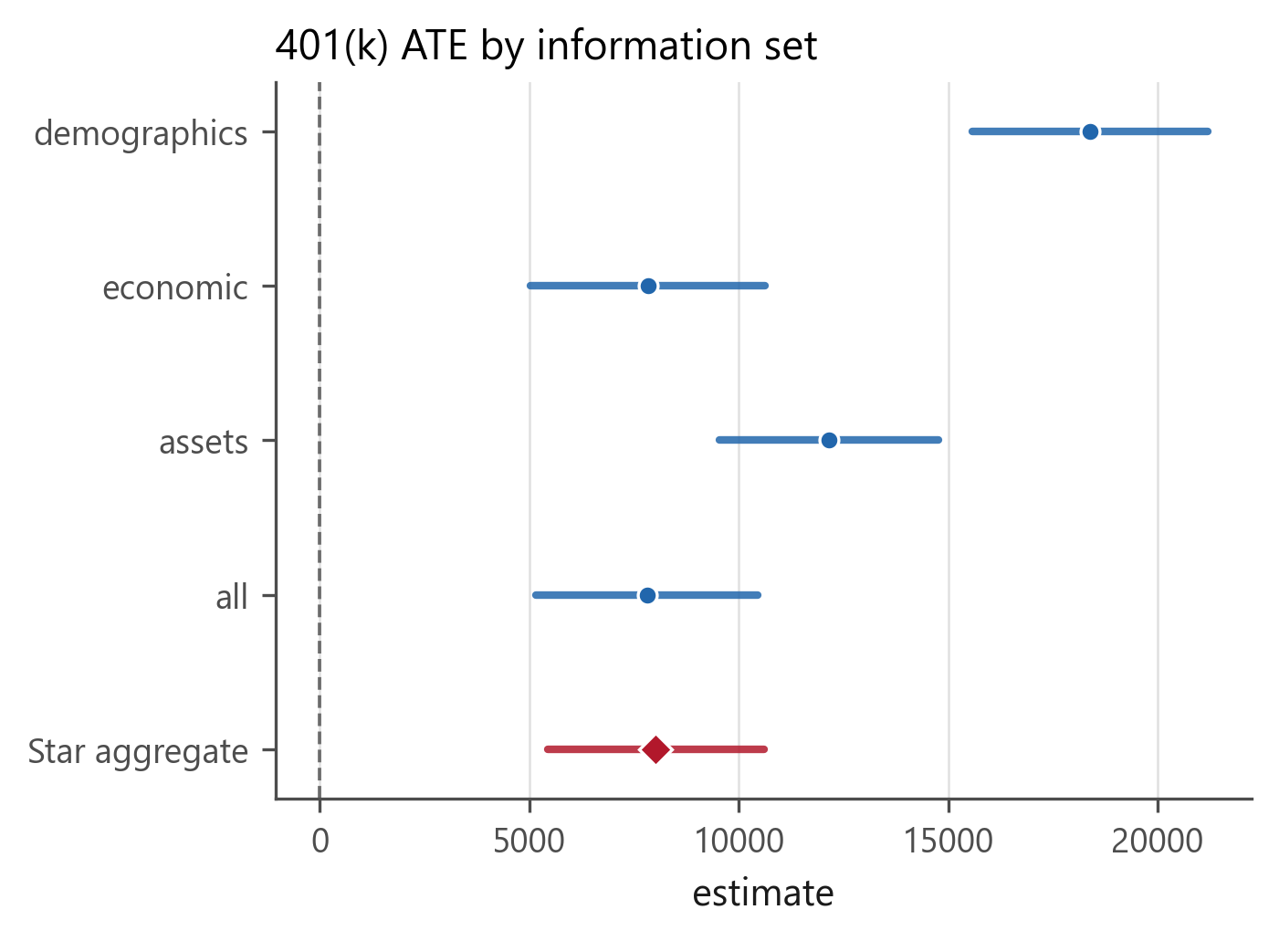
Estimates by information set

information set	estimate	std error	CI lower	CI upper
demographics	18,382	1,434	15,572	21,192
economic	7,828	1,432	5,021	10,636
assets	12,159	1,335	9,542	14,777
all	7,805	1,350	5,159	10,452
Star aggregate	8,019	1,315	5,442	10,597

Forest plot of the ATE by information set — Each row is a **different population target** $\theta_\lambda$, not a competing estimate of one number. Demographics alone barely adjusts anything; the economic block reproduces almost the whole adjustment. Income is doing the work — which is exactly why the parent paper benchmarks against it.

The scenario grid

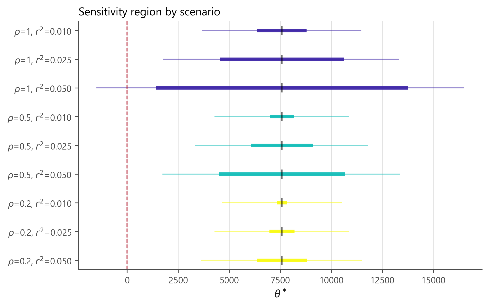
Sensitivity regions across nine scenarios — Thick bands are identified regions; thin whiskers add sampling uncertainty. The asymmetry the paper emphasises is visible: the *sign* is far more robust than the *magnitude*.

Reading the output

Practical guidance

Flexible in $X$ is not optional

On the 401(k) data a specification linear in the covariates returns about $4,900 — essentially plain OLS — against about $7,900 with splines. The treatment can be linear; the covariates usually cannot.

Trees cannot do derivatives

A piecewise-constant learner has zero derivative almost everywhere, so forests and boosting are inadmissible for AverageDerivative. pragdml warns you.

Star or convex aggregation?

Star costs $\log M$ and tolerates a huge menu; convex costs $\sqrt{M\log n}$ and needs $M\log n=o(\sqrt n)$. Call pooling_conditions and decide on your numbers.

Learn the two heads separately

The regression and the representer solve different problems and may select different candidates — the paper's own application does. Prediction quality alone does not summarise target preservation.

A warning worth heeding

RuntimeWarning: the cross-fitted representer has nu_hat^2 = -1.48 <= 0

$\hat\nu^2$ estimates $E[\alpha_0^2]>0$. A negative value means the Riesz fit has failed — almost always an over-wide basis. Do not report that estimate. Add ridge=, narrow the basis, or switch to AdditiveFeatures.

Beyond the papers

Cluster-robust variance	Section 5.1 requires it for repeated observations but supplies no estimator. `cluster=` keeps whole clusters inside a fold and adjusts the variance.
Multiplier bootstrap	The papers give only normal intervals; the influence values are already in hand.
Both parameterizations, kept apart	The two sources grid the same region differently. Conflating them would misstate every robustness value.
Rate diagnostics you can print	Eqs. (32), (35), (45) and (49) evaluated from the fitted objects, so the conditions are checkable rather than merely assumed.
Repeated cross-fitting	Median-aggregated across splits, as the parent paper's own application does.

Honest limitations

The paper's own application is not reproducible here. Its product data is scraped from Keepa.com and is not public. pragdml reproduces the paper's arithmetic — all eighteen Table 3 endpoints to the last printed digit — but not its data.
No reference implementation exists for the target paper. Compatibility evidence is the ATE special case against DoubleML, plus the parent paper's published numbers.
The sensitivity parameters are assumptions. The package estimates the scale; the strengths and the alignment are yours to defend.
Oracle bounds are rate shapes. The universal constants are unspecified in the paper; reported values use $C=1$.

References

A. Aradillas Fernández, V. Chernozhukov, C. Cinelli, S. Klaassen, W. Newey, M. Spindler, J. Teichert-Kluge & S. Vijaykumar (2026). Pragmatic DML with AI-Learned Representations. arXiv:2610.01935
V. Chernozhukov, C. Cinelli, W. K. Newey, A. Sharma & V. Syrgkanis (2026). Long Story Short: Omitted Variable Bias in Causal Machine Learning. Review of Economics and Statistics. doi:10.1162/REST.a.1705
V. Chernozhukov, W. K. Newey & R. Singh (2022). Automatic Debiased Machine Learning of Causal and Structural Effects. Econometrica 90(3):967–1027. doi:10.3982/ECTA18515
V. Chernozhukov, D. Chetverikov, M. Demirer, E. Duflo, C. Hansen, W. Newey & J. Robins (2018). Double/Debiased Machine Learning. The Econometrics Journal 21(1):C1–C68. doi:10.1111/ectj.12097
S. Vijaykumar (2021). Localization, Convexity, and Star Aggregation. NeurIPS 34:4570–4581. arXiv:2105.08866
T. Liang, A. Rakhlin & K. Sridharan (2015). Learning with Square Loss: Localization through Offset Rademacher Complexity. COLT.
J.-Y. Audibert (2007). Progressive Mixture Rules are Deviation Suboptimal. NeurIPS 20.
C. Cinelli & C. Hazlett (2020). Making Sense of Sensitivity. JRSS-B 82(1):39–67. doi:10.1111/rssb.12348

All DOIs verified 17 October 2026.

Citing

@software{roudane2026pragdml,
  author  = {Roudane, Merwan},
  title   = {pragdml: Pragmatic double machine learning with AI-learned representations},
  year    = {2026},
  version = {0.1.1},
  url     = {https://github.com/merwanroudane/PragDML}
}

Please also cite the papers the package implements (references 1 and 2).

You assume	The interval covers	At what variance
Assumption 1 only	\(\theta_\lambda\), the representation's own target	the short score's
+ target adaptivity (Def. 1)	\(\theta^{*}\), the causal parameter	the short score's
+ adaptive efficiency (Def. 2)	\(\theta^{*}\)	the semiparametric bound

Term	Meaning	Identified?
\(S^2=E[(Y-g_0)^2]\,E[\alpha_0^2]\)	the scale of any possible bias	yes — estimated by DML
\(C_Y^2\)	share of residual outcome variation the omitted information could explain	no — you assume it
\(C_D^2\)	the same for the balancing weight	no — you assume it
\(\rho\in[-1,1]\)	alignment of the two omitted components	no — you assume it

`ATE`	\(E[g(1,X)-g(0,X)]\) — binary treatment
`AverageDerivative`	\(E[\partial_d g(d,X)\|_{d=D}]\) — continuous treatment (Eq. 67)
`ATT`	a ratio target, with a delta-method correction
`AveragePotentialOutcome`, `WeightedATE`, `PolicyEffect`	further members of the Riesz-linear class