asycaus v 1.0.0
Asymmetric Granger-causality suite for Python and Stata.


Author Dr Merwan Roudane · merwanroudane920@gmail.com
📦 PyPI: https://pypi.org/project/asycaus/ · 💻 GitHub: https://github.com/merwanroudane/asycaus · 📊 Stata twin:
ssc install asycaus
0 · Quick links
- Install (Python):
pip install asycaus→ pypi.org/project/asycaus - Install (Stata):
ssc install asycaus - Source code: https://github.com/merwanroudane/asycaus
- Issues / bug reports: https://github.com/merwanroudane/asycaus/issues
- Executed notebook: full_demo.html
- API reference: SYNTAX.md
1 · Theory in 5 minutes
1.1 Granger non-causality
Variable x does not Granger-cause variable y if the past of x does not help predict y once the past of y is conditioned on. In a VAR(p):
\[y_t = c + \sum_{r=1}^{p} a_{yy,r}\,y_{t-r} + \sum_{r=1}^{p} a_{yx,r}\,x_{t-r} + \varepsilon_{y,t}\]H0: ayx,1 = ⋯ = ayx,p = 0.
The conventional Wald statistic asks whether the sum of all causal effects is zero. This makes one strong assumption: positive and negative innovations in x matter identically for y.
1.2 Why asymmetry matters
In financial markets, that assumption is almost always wrong:
- Investors react more strongly to bad news than good (loss aversion, Akerlof, Spence, Stiglitz).
- Asset-price floors at zero make pos/neg shocks structurally different.
- Sticky-price models give different cost pass-through up vs. down.
If we lump positive and negative shocks together, we wash out any asymmetry and risk a false “no causality” conclusion when in fact one direction is causal.
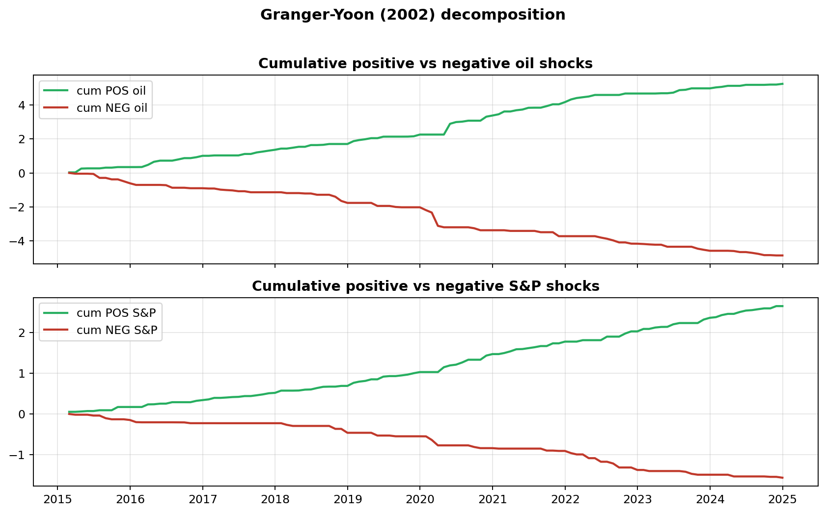
1.3 Granger and Yoon (2002) decomposition
Each variable is decomposed into the cumulative sum of its positive and cumulative sum of its negative innovations:
\[x_t^+ = \sum_{i=1}^{t} \max(\Delta x_i, 0), \qquad x_t^- = \sum_{i=1}^{t} \min(\Delta x_i, 0).\]We then test for Granger causality separately on each pair: x+ → y+ and x− → y−.
1.4 The seven tests in this package
| # | Test | Method paper |
|---|---|---|
| 1 | Static asymmetric + leverage bootstrap | Hatemi-J (2012); Hacker & Hatemi-J (2006, 2012) |
| 2 | Dynamic (rolling / recursive) | Hatemi-J (2021) |
| 3 | Fourier-augmented asymmetric TY | Nazlioglu et al. (2016); Pata (2020) |
| 4 | Frequency-domain (Breitung-Candelon) on Pos/Neg components | Bahmani-Oskooee, Chang & Ranjbar (2016) |
| 5 | Quantile asymmetric (+ Fourier) | Fang, Wang, Shieh & Chung (2026) |
| 6 | Efficient SUR (Pos / Neg / Joint / Pos = Neg) | Hatemi-J (2024) |
| 7 | Unified battery + dashboard | this package |
All seven share a single HJC (Hatemi-J 2003) information criterion for lag selection by default, with AIC / AICC / SBC / HQC also available.
2 · Installation
Python
pip install asycaus
# or from source:
pip install git+https://github.com/merwanroudane/asycaus.git
Requires Python ≥ 3.9. Dependencies (installed automatically): numpy,
scipy, pandas, matplotlib, rich.
Stata
ssc install asycaus
help asycaus
Requires Stata ≥ 14.
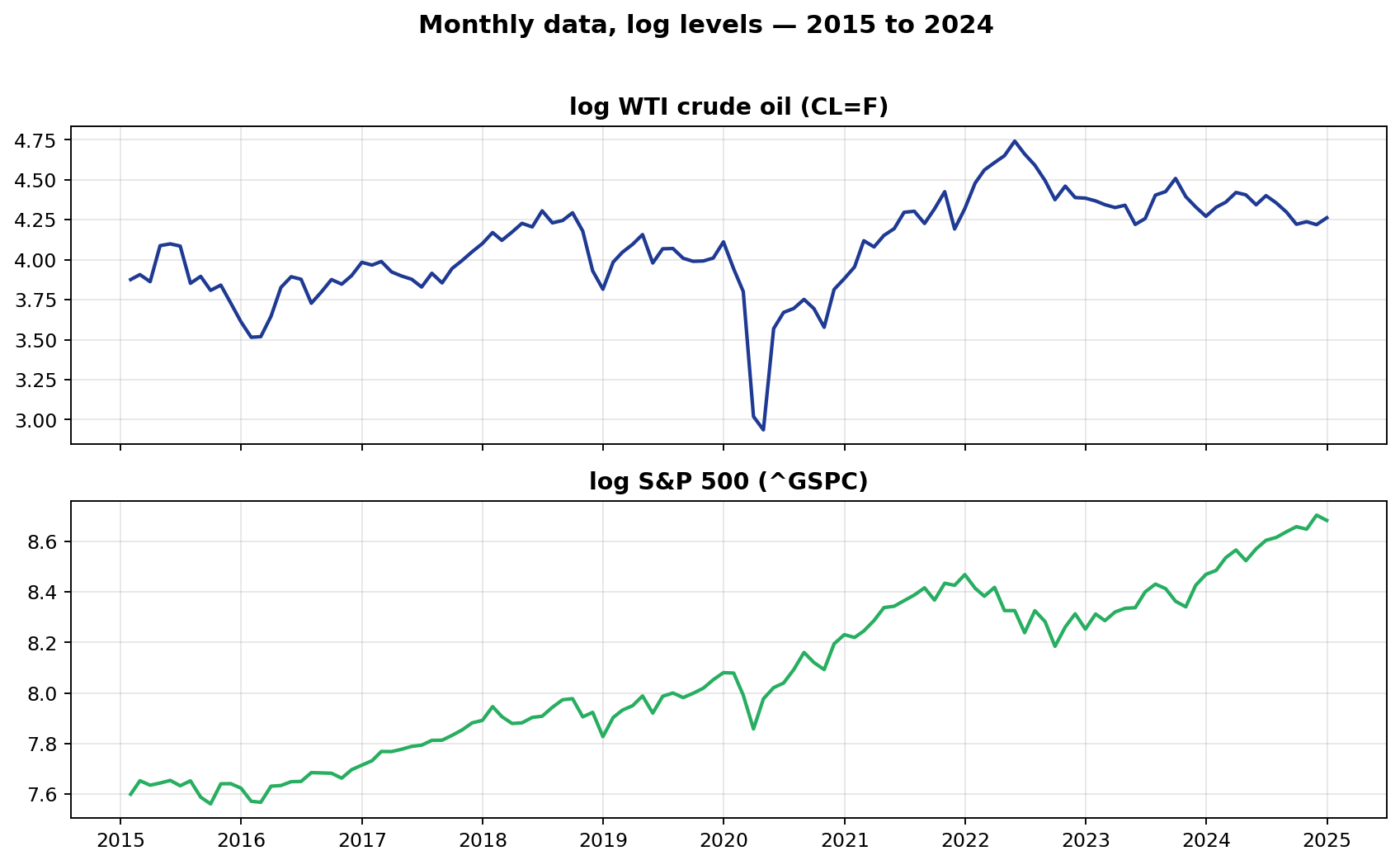
3 · Practical example — oil and the S&P 500
The block below is the empirical study from the executed notebook
(full_demo.html), which downloads daily WTI crude
and S&P 500 closes from Yahoo Finance, aggregates to monthly log levels and
runs every test in the library. Every figure on this page comes from that
notebook (see also docs/tables/ and docs/figures/).
3.1 Data
import yfinance as yf, numpy as np, asycaus

raw = yf.download(['CL=F', '^GSPC'], start='2015-01-01', end='2024-12-31',
                  progress=False, auto_adjust=True)['Close'].dropna()
monthly = raw.resample('M').last().apply(np.log).dropna()
y = monthly['^GSPC'].to_numpy()   # ln S&P 500
x = monthly['CL=F'].to_numpy()    # ln WTI crude oil
3.2 Cumulative pos / neg shocks
Y = np.column_stack([y, x])
C_pos = asycaus.pos_neg_components(Y, positive=True)
C_neg = asycaus.pos_neg_components(Y, positive=False)
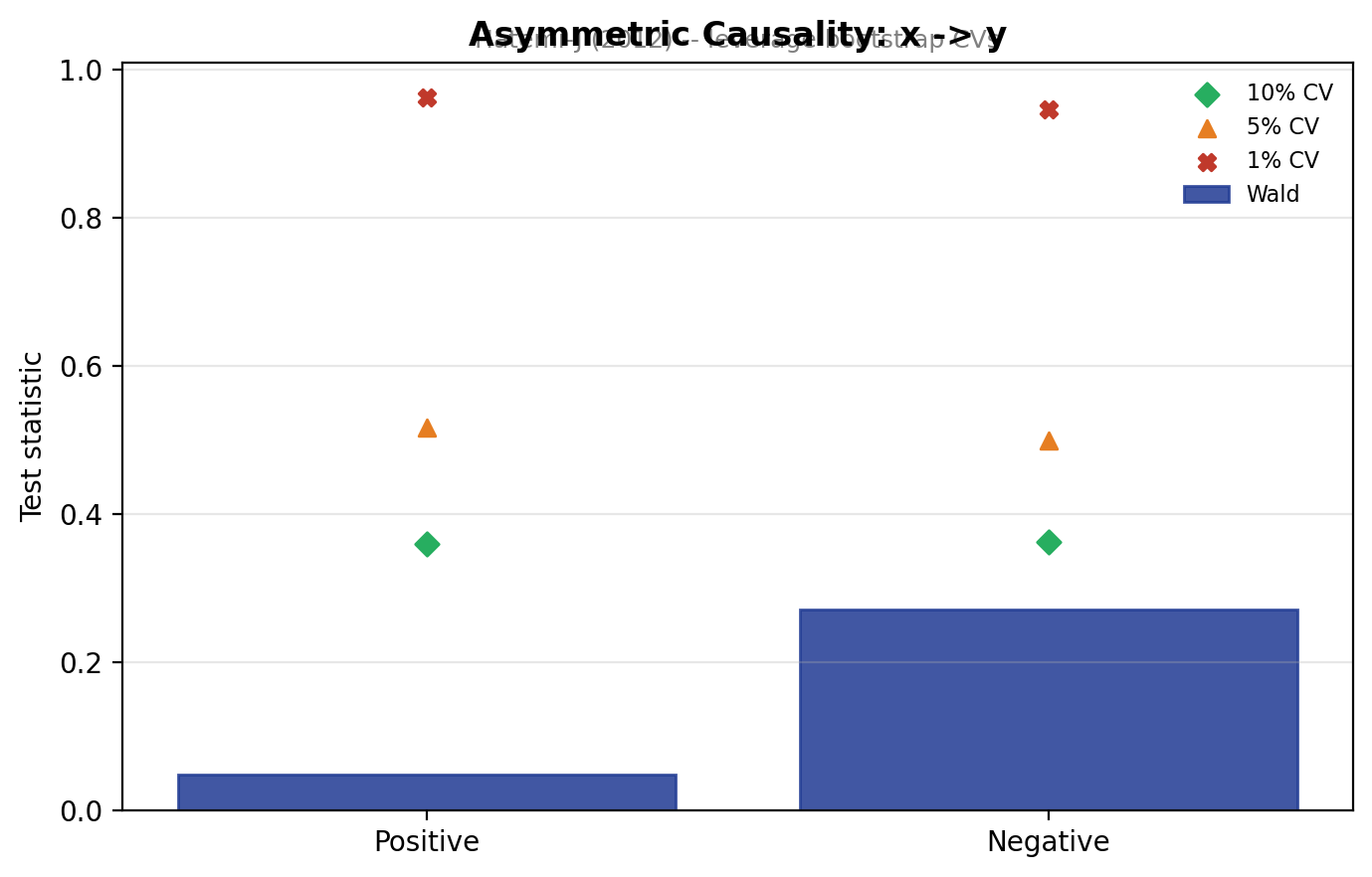
3.3 Static asymmetric — Hatemi-J (2012)
asycaus.static(y, x, shock='both', max_lag=6, boot=500)
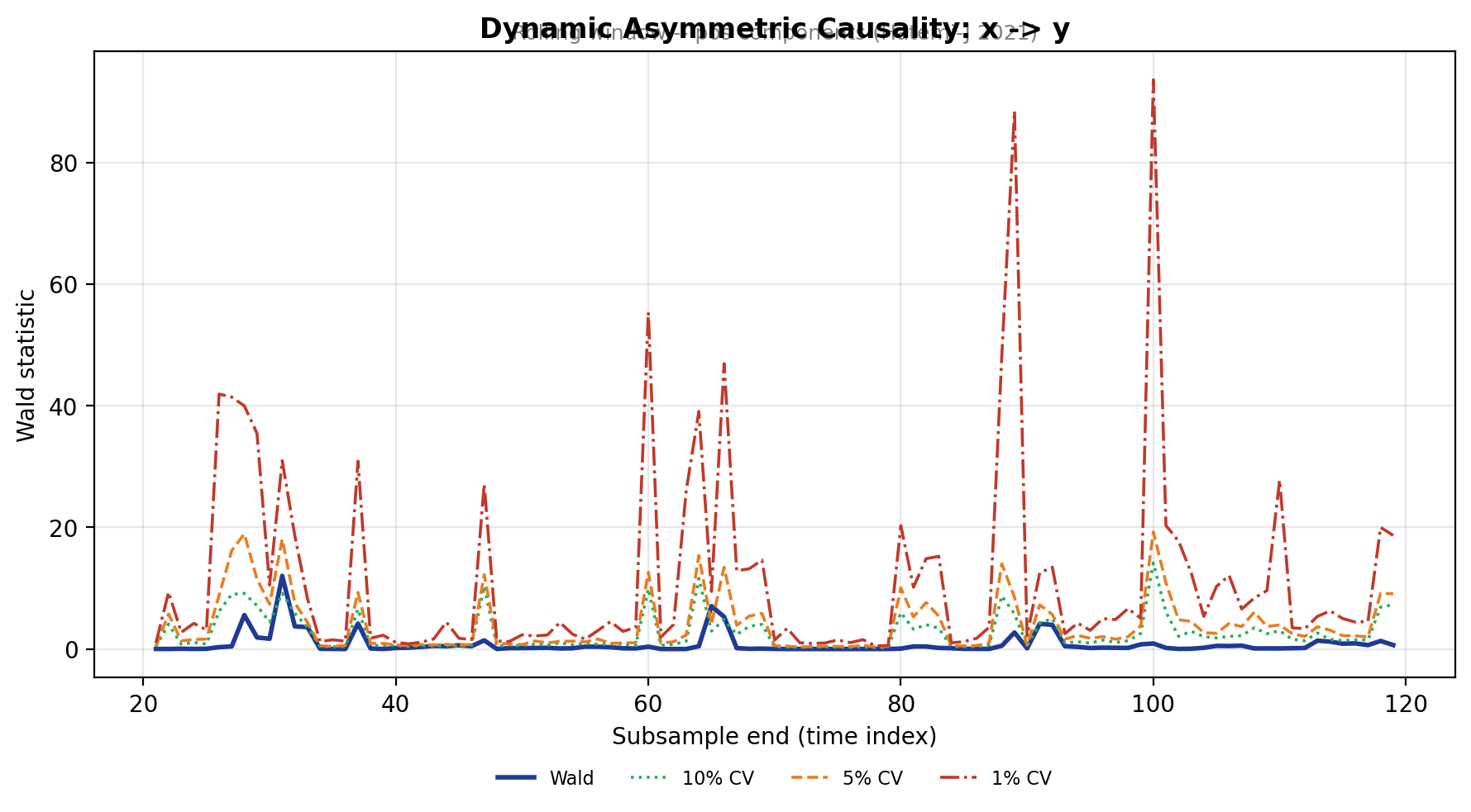
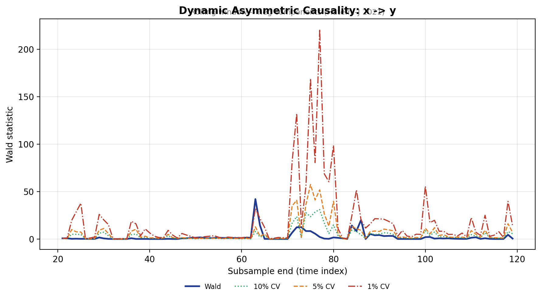
3.4 Dynamic asymmetric — Hatemi-J (2021)
asycaus.dynamic(y, x, shock='pos', mode='rolling', max_lag=3, boot=120)
asycaus.dynamic(y, x, shock='neg', mode='rolling', max_lag=3, boot=120)
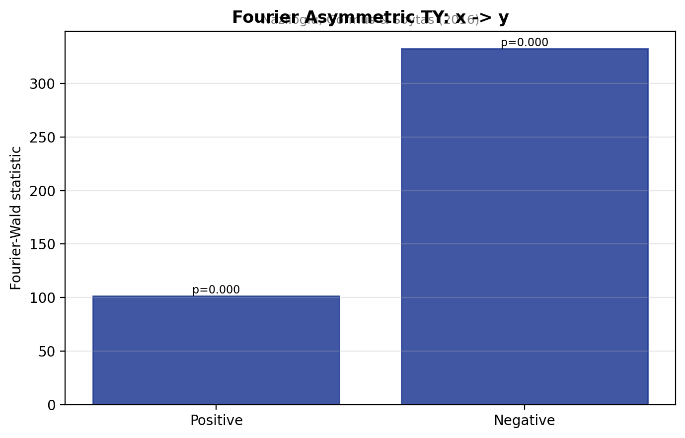
3.5 Fourier-augmented TY — Nazlioglu et al. (2016)
Smooth structural breaks (Covid-19 crash, 2022 Ukraine invasion, etc.) are absorbed by sin/cos terms.
asycaus.fourier(y, x, shock='both', kmax=4, form='single', max_lag=6)
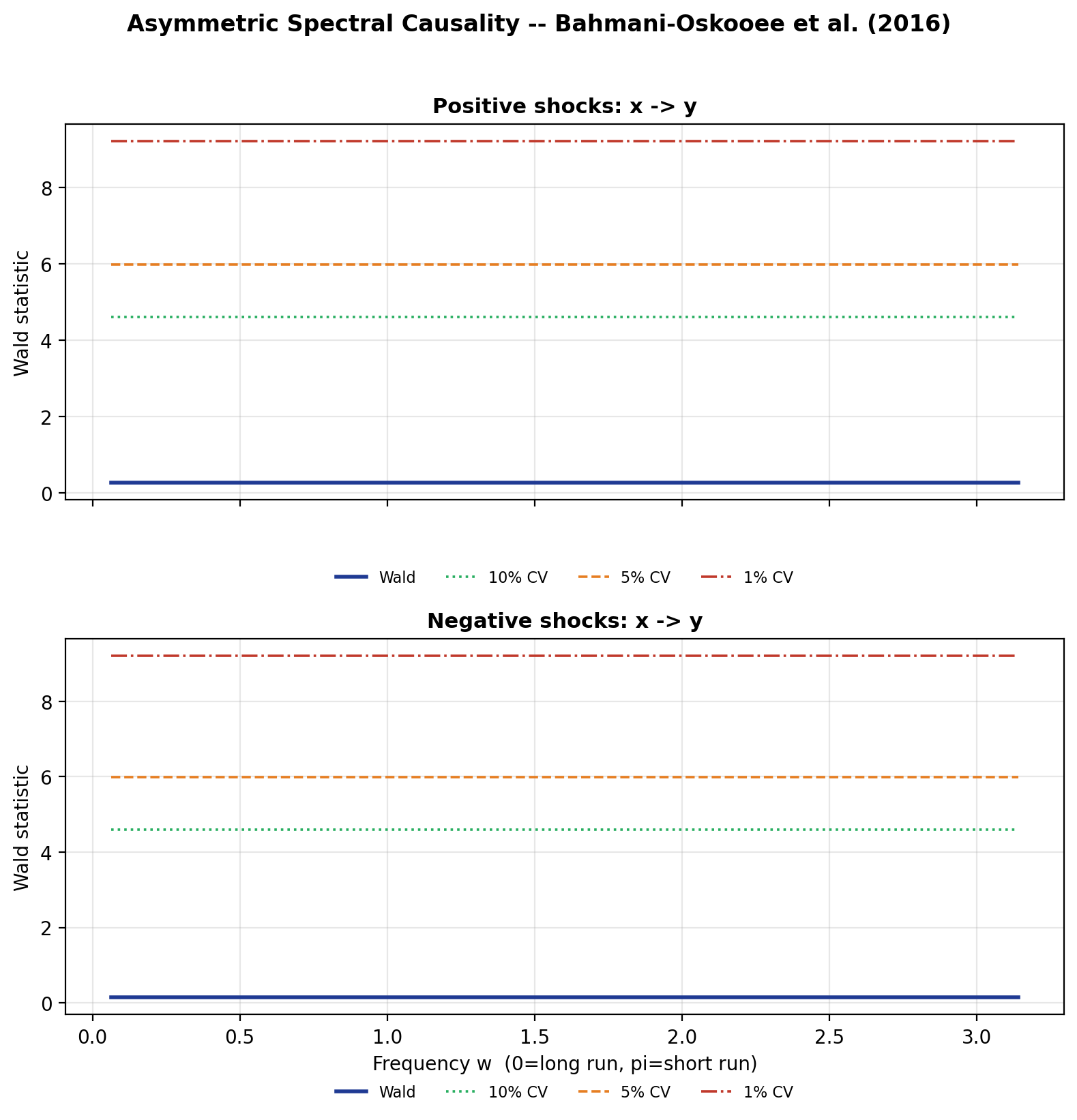
3.6 Frequency-domain — Bahmani-Oskooee et al. (2016)
asycaus.spectral(y, x, shock='both', nfreq=50, max_lag=6)
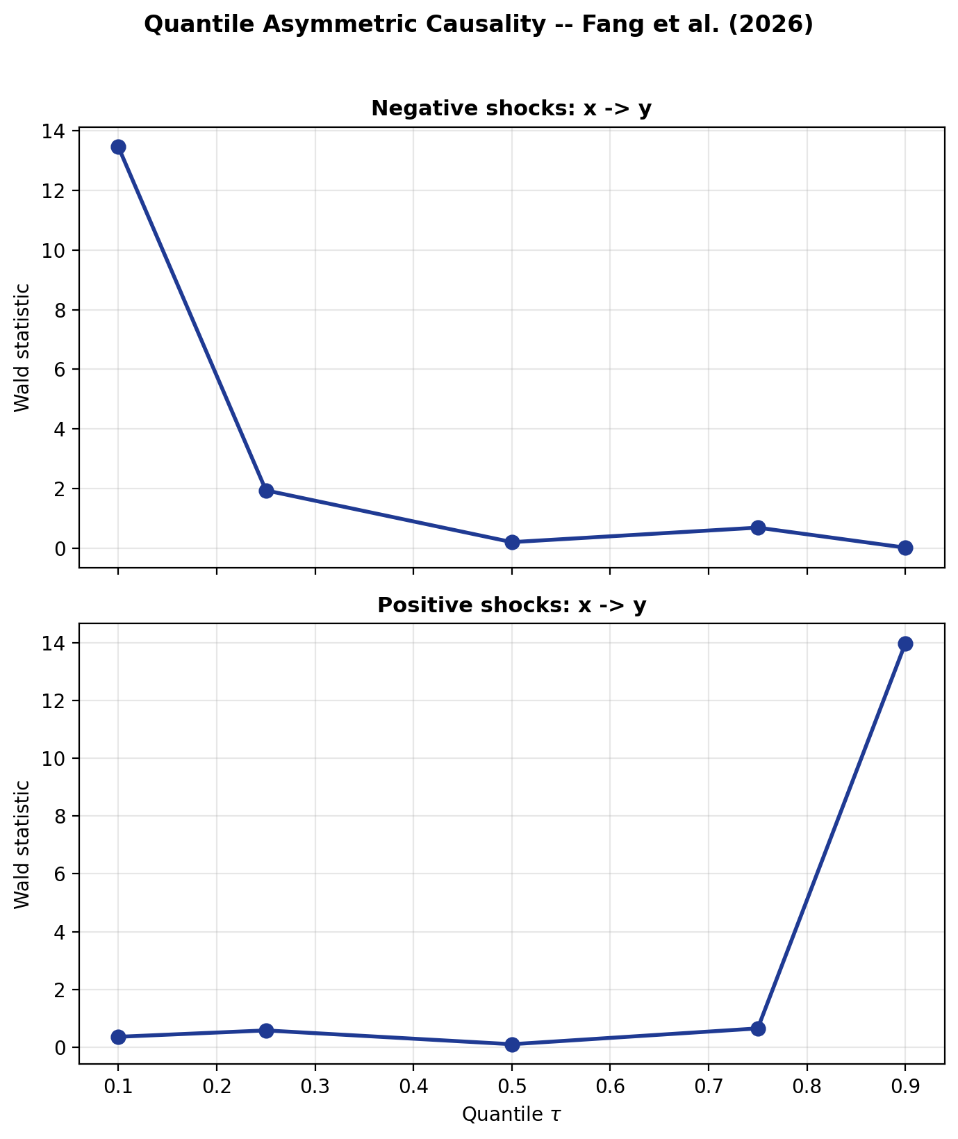
3.7 Quantile — Fang et al. (2026)
asycaus.quantile(y, x, shock='both',
                 quantiles=(0.1, 0.25, 0.5, 0.75, 0.9),
                 max_lag=4, fourier=True, kmax=2)
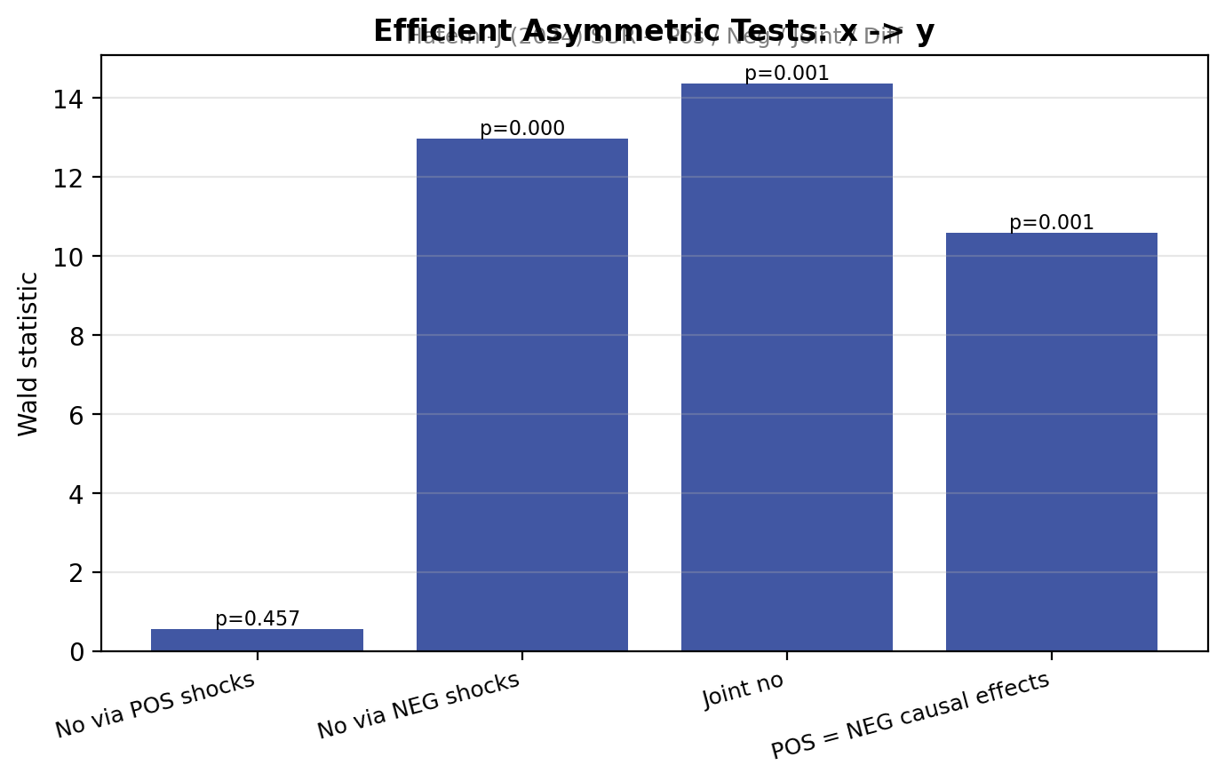
3.8 Efficient SUR — Hatemi-J (2024)
The decisive test: does the positive-shock causal coefficient differ from the negative-shock causal coefficient? Rejection ⇒ formal evidence of asymmetric causation.
asycaus.efficient(y, x, max_lag=6)
3.9 Unified summary
| Test | Shock | Statistic | p-value | Decision |
|---|---|---|---|---|
| Static (Hatemi-J 2012) | Pos | 0.048 | 0.826 | Fail to reject |
| Static (Hatemi-J 2012) | Neg | 0.271 | 0.603 | Fail to reject |
| Fourier (Nazlioglu 2016) | Pos | 101.52 | < 0.001 | Reject |
| Fourier (Nazlioglu 2016) | Neg | 332.32 | < 0.001 | Reject |
| Efficient Pos only (HJ 2024) | Pos | 0.554 | 0.457 | Fail to reject |
| Efficient Neg only (HJ 2024) | Neg | 12.962 | < 0.001 | Reject |
| Efficient Joint (HJ 2024) | both | 14.363 | 0.001 | Reject |
| Efficient Pos = Neg (HJ 2024) | diff | 10.575 | 0.001 | Reject |
The headline finding is the Hatemi-J (2024) Pos = Neg test rejecting at the 1% level (W = 10.575, p = 0.001) — formal evidence that crude-oil shocks affect the S&P 500 asymmetrically over 2015–2024. Negative oil shocks have a significant causal impact whereas positive ones do not, a finding that the conventional symmetric Granger test cannot detect.
4 · Documented API
Every function has a one-line summary in the README and a full description in
docs/SYNTAX.md.
import asycaus
asycaus.static    (y, x, ...)   # Hatemi-J (2012)
asycaus.dynamic   (y, x, ...)   # Hatemi-J (2021)
asycaus.fourier   (y, x, ...)   # Nazlioglu, Gormus & Soytas (2016)
asycaus.spectral  (y, x, ...)   # Bahmani-Oskooee, Chang & Ranjbar (2016)
asycaus.quantile  (y, x, ...)   # Fang, Wang, Shieh & Chung (2026)
asycaus.efficient (y, x, ...)   # Hatemi-J (2024)
asycaus.all_tests (y, x, ...)   # full battery
asycaus.pos_neg_components(Y, positive=True)   # Granger-Yoon (2002)
Each returns a Result dataclass with three things:
.table—pandas.DataFrameof the numerical output.print()— re-render the boxedrichtable.plot(save="filename.png")— re-render the publication-quality plot
5 · Companion Stata package
A 1-to-1 Stata twin of this library is available on SSC with the same name:
ssc install asycaus
help asycaus
asycaus static  dln_inv dln_inc, boot(500) shock(both)
asycaus dynamic dln_inv dln_inc, rolling boot(150)
asycaus all     dln_inv dln_inc, maxlag(4) boot(300)
The Stata version produces identical numerical output and analogous publication-quality graphs.
6 · References
- Bahmani-Oskooee, M., Chang, T., & Ranjbar, O. (2016). Asymmetric causality using frequency-domain and time-frequency-domain (wavelet) approaches. Economic Modelling, 56, 66–78.
- Breitung, J., & Candelon, B. (2006). Testing for short- and long-run causality. Journal of Econometrics, 132, 363–378.
- Enders, W., & Lee, J. (2012). The flexible Fourier form and DF-type unit root tests. Economics Letters, 117(1), 196–199.
- Fang, H., Wang, C.-H., Shieh, J. C. P., & Chung, C.-P. (2026). The asymmetric Granger causality between banking-sector and stock-market development and economic growth in quantiles considering Fourier. Applied Economics, 58(20), 3822–3838.
- Granger, C. W. J., & Yoon, G. (2002). Hidden cointegration. UCSD Discussion Paper 2002-02.
- Hacker, R. S., & Hatemi-J, A. (2006). Tests for causality between integrated variables using asymptotic and bootstrap distributions. Applied Economics, 38(13), 1489–1500.
- Hacker, R. S., & Hatemi-J, A. (2012). A bootstrap test for causality with endogenous lag length choice. Journal of Economic Studies, 39(2), 144–160.
- Hatemi-J, A. (2003). A new method to choose optimal lag order in stable and unstable VAR models. Applied Economics Letters, 10(3), 135–137.
- Hatemi-J, A. (2012). Asymmetric causality tests with an application. Empirical Economics, 43, 447–456.
- Hatemi-J, A. (2021). Dynamic Asymmetric Causality Tests with an Application. arXiv 2106.07612.
- Hatemi-J, A. (2024). Efficient Asymmetric Causality Tests. arXiv 2408.03137.
- Koenker, R. (2005). Quantile Regression. Cambridge University Press.
- Nazlioglu, S., Gormus, N. A., & Soytas, U. (2016). Oil prices and REITs: gradual-shift causality. Energy Economics, 60, 168–175.
- Pata, U. K. (2020). How is COVID-19 affecting environmental pollution in US cities? Evidence from asymmetric Fourier causality test. Air Quality, Atmosphere & Health, 13, 1149–1155.
- Phillips, P. C. B., Shi, S., & Yu, J. (2015). Testing for multiple bubbles. International Economic Review, 56(4), 1043–1078.
- Toda, H. Y., & Yamamoto, T. (1995). Statistical inference in vector autoregressions with possibly integrated processes. Journal of Econometrics, 66, 225–250.
7 · Citation
@software{roudane2026asycaus,
  author = {Roudane, Merwan},
  title  = {asycaus: Asymmetric Granger-causality suite for Python and Stata},
  year   = {2026},
  url    = {https://github.com/merwanroudane/asycaus},
  version= {1.0.0}
}