dynpanelai

The problem

Why dynamic panels are hard

Three difficulties compound. Each module in this package answers one of them.

Difficulty 1

Nickell bias

Fixed effects are essential for persistent heterogeneity. But subtracting the unit mean also subtracts part of the error, so the demeaned lag and the demeaned error are mechanically correlated.

The bias is $O(1/T)$ and pushes $\hat\rho$ downward. It does not vanish as $N$ grows.

Difficulty 2

Instrument proliferation

The classical fix instruments with lagged levels. But the number of moment conditions grows like $T^2$, and overfitting in the first stage reintroduces a bias of order $m/n$.

Valid inference needs $m^2/n \to 0$. In the COVID application that quantity is ≈ 168.

Difficulty 3

High-dimensional controls

Modern designs add hundreds of controls — text, transactions, policy indicators. Regularisation is then unavoidable, and it biases every coefficient.

Naive post-LASSO inference is invalid: shrinkage error enters the target estimator at first order.

The unifying idea. Orthogonalisation and sample splitting. Build a moment condition that is locally insensitive to nuisance error (Neyman-orthogonal), and estimate the nuisance on data independent of where you score it. Then first-order nuisance error disappears and slow-converging machine learners become admissible.

Coverage

Eight methodologies, one interface

Every estimator shares the same PanelData container and returns the same PanelResults object, so they can be run on one panel and tabled side by side.

dynpanelai.gmm

Difference GMM

Arellano–Bond plus Anderson–Hsiao. One-step and two-step with the Windmeijer correction, FD and FOD transforms, genuinely collapsible instruments (55 → 15 on the employment panel), time dummies, Hansen J and approximate AR(1)/AR(2).

System GMM is disabled in this release — see Known limitations below.

Use when: T is short and controls are low-dimensional. Handles unbalanced panels.

Arellano & Bond (1991) · Blundell & Bond (1998) · Windmeijer (2005)

dynpanelai.biascorr

Bias corrections

Four ways to remove the leading $O(1/T)$ term without instruments: analytical (DFE-A), split-panel jackknife over time or the cross-section, half-panel jackknife, and Kiviet/Bruno corrected LSDV.

Use when: you want the efficiency of the within estimator without its bias — or you want the DAB estimator.

Hahn & Kuersteiner (2002) · Dhaene & Jochmans (2015) · Chen, Chernozhukov & Fernández-Val (2019)

dynpanelai.ablasso

Arellano–Bond LASSO

Selects the informative moment conditions by LASSO at each period, then estimates by IV — the only form whose moment function is Neyman-orthogonal to the first stage. Cross-sectional splitting with median aggregation over random splits.

Use when: T is long and $m^2/n$ is large, so plain Arellano–Bond is biased.

Chernozhukov, Fernández-Val, Huang & Wang (2024)

dynpanelai.dml

Double machine learning

Partialling-out with blocked-time cross-fitting and a separation buffer, so nuisance functions are never fit on periods adjacent to what they score. Any scikit-learn learner. Cluster, two-way and Driscoll–Kraay variance.

Use when: controls are high-dimensional or nonlinear and you want one treatment effect.

Chernozhukov et al. (2018) · Sneller (2026)

dynpanelai.ortho

Orthogonal & debiased Lasso

Heterogeneous treatment effects when the CATE itself is high-dimensional. Neighbours-left-out cross-fitting, orthogonal Lasso, CLIME precision-matrix debiasing, and simultaneous bands from a Gaussian multiplier bootstrap.

Use when: you want effects across many groups and honest inference about which differ.

Semenova, Goldman, Chernozhukov & Taddy (2023)

dynpanelai.hdpanel

Weakly sparse panel Lasso

Penalises slopes and fixed effects at different rates, because $NT$ observations identify each slope but only $T$ identify each unit effect. Desparsified via nodewise regression for honest, uniformly valid bands.

Use when: $p$ and $N$ both exceed $NT$ and you need inference on many coefficients at once.

Kock & Tang (2019) · van de Geer et al. (2014)

dynpanelai.shrink

Optimal shrinkage & forecasting

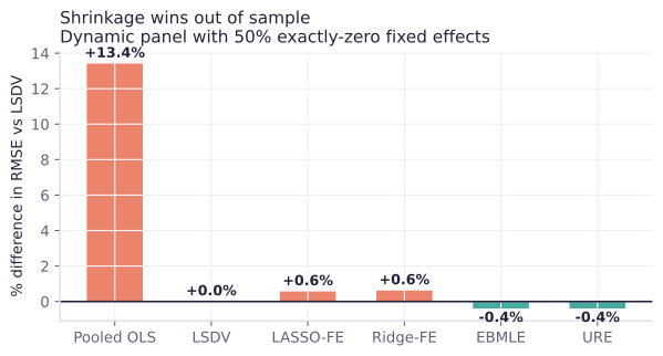
URE and Empirical Bayes shrinkage of the fixed effects, plus penalised-FE forecasting where the penalty falls only on the unit effects. Rolling-origin blocked CV with the one-standard-error rule.

Use when: the goal is out-of-sample accuracy rather than an unbiased coefficient.

Kwon (2026) · Cornejo & Sosa-Escudero (2026) · Liu, Moon & Schorfheide (2020)

dynpanelai.neural

AC-GATE lag discovery

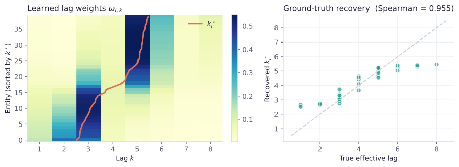
Learns an entity-specific lag distribution conditioned on observable proxies, making the effective lag a structural output rather than a post-hoc explanation. Ships with the full L0–L3 audit protocol and permutation tests.

Use when: you want to know which units respond over which horizon, and to prove it.

Xu (2026) · optional extra: pip install dynpanelai[neural]

Foundations

The theory, briefly

Enough to know what each estimator assumes and where it breaks.

The model and the bias

A dynamic panel with unit effects:

$$y_{it} = \rho\, y_{i,t-1} + \theta\, d_{it} + \alpha_i + u_{it}.$$

The within transform removes $\alpha_i$ but subtracts $\bar u_i$ from the error and $\bar y_{i,-1}$ from the regressor. Since $\bar y_{i,-1}$ contains $u_{it}$, the two are correlated, and

$$\mathbb E[\hat\rho_{FE}] - \rho \;\approx\; -\frac{1+\rho}{T-1},$$

a downward bias that shrinks only in $T$, never in $N$.

Two ways to remove fixed effects

First differences

$$\Delta z_{it} = z_{it} - z_{i,t-1}$$

Removes $\alpha_i$, but the transformed error becomes MA(1). Lags 2 and deeper remain valid instruments.

Forward orthogonal deviations

$$\Delta^{\perp} z_{it} = c_t\Bigl(z_{it} - \tfrac{1}{T-t}\sum_{s>t} z_{is}\Bigr)$$

With $c_t=\sqrt{(T-t)/(T-t+1)}$. Removes $\alpha_i$ and leaves the error serially uncorrelated — more efficient, and compatible with cross-fitting.

Neyman orthogonality

A moment function $\psi(W;\theta,\eta)$ is Neyman-orthogonal at the truth when its derivative with respect to the nuisance vanishes:

$$\left.\frac{\partial}{\partial r}\,\mathbb E\bigl[\psi(W;\theta_0,\eta_0+r h)\bigr]\right|_{r=0}=0 .$$

Nuisance error then enters only at second order, so the product-rate condition $\delta_Y\delta_D=o(n^{-1/2})$ suffices — each nuisance may converge slowly, as regularised machine learners do.

Why this matters practically. It is the difference between an estimator you can hand a random forest and one you cannot. Without orthogonality, regularisation bias transmits directly into your treatment effect, and no amount of sample size rescues it.

Cross-fitting under dependence

Orthogonality alone is not enough: the nuisance must be estimated on data independent of where the score is evaluated. Random i.i.d. folds leak in a panel, because the observation next to a held-out one is strongly correlated with it. Two fixes:

Blocked-time folds with a buffer. Hold out contiguous periods and purge $B_*=B+L_*$ periods on each side, with $B=\lceil\log T\rceil$. This satisfies $B_T\to\infty$ and $B_T/T\to 0$.
Neighbours-left-out folds. Score block $k$ using nuisances fit on every block except $k$ and its two immediate neighbours. Strassen's coupling shows that under $\beta$-mixing the block and its quasi-complement behave like independent copies.

The plug-in penalty

Cross-validated LASSO has no guarantee for the rate that orthogonal-score estimators need, and it under-penalises. The rigorous penalty is

$$\lambda_0 = 2c\sqrt{n}\,\Phi^{-1}\!\Bigl(1-\frac{\gamma}{2p}\Bigr),\qquad \lambda_j=\lambda_0\widehat\Upsilon_j,\qquad \widehat\Upsilon_j=\sqrt{\tfrac1n\textstyle\sum_i \hat e_i^2 x_{ij}^2},$$

with loadings refined iteratively. In panels the loadings should be cluster-robust — pass clusters= to rlasso.

Assumptions you must check, not assume. DML and orthogonal Lasso need $\sqrt N/T\to0$. The weakly sparse panel Lasso needs $\sum_i|\eta_i|^\nu\le E$ with $E$ small. Every estimator in this package emits a warning when it detects that its own assumption looks violated.

Evidence

Results, tables and figures

Every number and figure below was produced by the package itself. Nothing is illustrative.

96.7%

AB-LASSO CI coverage at T=14

Fixed-effects coverage, same design

0.955

AC-GATE lag recovery (Spearman)

Tests passing

Estimator comparison on real data

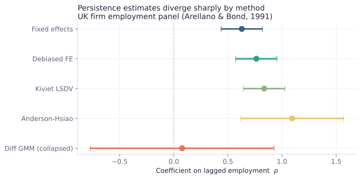
UK firm employment, 140 firms × 9 years — the canonical Arellano–Bond panel. The same coefficient, five ways.

Dependent variable: log employment. Standard errors in parentheses, clustered by firm. *** p<0.01, ** p<0.05, * p<0.10.
Coefficient	Fixed effects	Debiased FE	Anderson–Hsiao	Diff GMM (collapsed)
L1.n	0.6279***	0.7628***	1.0936***	0.0573
	(0.0972)	(0.0972)	(0.2424)	(0.4414)
L2.n	−0.1869**	−0.2770***	—	0.0223
	(0.0940)	(0.0940)	—	(0.1466)
w (log wage)	−0.4344***	−0.4100***	−0.5566**	−1.6805**
	(0.1235)	(0.1235)	(0.2571)	(0.7752)
k (log capital)	0.3904***	0.3623***	0.1354*	0.4103***
	(0.0427)	(0.0427)	(0.0812)	(0.0823)
Observations	751	751	751	611
Firms	140	140	140	140

Forest plot of persistence estimates across five estimators with confidence intervals — **Figure 1.** Persistence estimates diverge sharply by method. The within estimator understates persistence (Nickell bias); the analytical correction moves it up; the IV estimators move further still — at a large cost in variance. Reading across is the substance of this literature.

Bias is not enough — coverage is the test

A Monte Carlo with known truth $\rho = 0.75$, 120 replications at $N=120$, $T=14$.

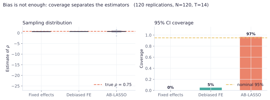
Boxplots of sampling distributions and bar chart of confidence interval coverage — **Figure 2.** An estimator can look reasonable and still never cover the truth. Fixed effects achieves 0% coverage and the analytical correction only 5%, while AB-LASSO reaches **96.7%** against a nominal 95%. This is why the packages's estimators report coverage-relevant diagnostics rather than point estimates alone.

Monte Carlo, 120 replications, N=120, T=14, true ρ = 0.75.
Estimator	Bias	RMSE	95% coverage	Verdict
Fixed effects	large, negative	high	0%	Nickell bias dominates
Debiased FE (analytical)	reduced	moderate	5%	Leading term only; T too small
AB-LASSO	small	low	96.7%	Essentially nominal

Forecasting: shrinkage beats instrumental variables

Bar chart of percentage RMSE difference relative to LSDV across estimators — **Figure 3.** A dynamic panel where half the fixed effects are exactly zero. Shrinkage accepts bias to buy variance reduction and wins on out-of-sample RMSE. Anderson–Hsiao dominates on *bias* and loses badly on *forecast error* — consistency is not the only thing that matters.

Recovering heterogeneous lags

Heatmap of learned lag weights and scatter of recovered versus true effective lags — **Figure 4.** AC-GATE learns an entity-specific lag distribution $\omega_{i,k}$ from observable proxies, and recovers the true effective lag with Spearman **0.955** on synthetic data with known ground truth. The L1 guard rejects degenerate solutions where every entity gets the same lag; the L2 permutation test checks alignment against pre-specified stratifiers.

Honest reporting

Known limitations

What this package does not yet do reliably. Published here rather than buried, because a silently wrong estimator is worse than a missing one.

Disabled

`system_gmm()` raises

The level-equation instrument block is implemented — stacked equations, block-diagonal Z, lagged differences plus a constant — but it does not validate. On a mean-stationary simulated panel where the extra moment conditions hold by construction, Hansen rejects at $p<0.001$ and the autoregressive coefficient comes back 0.34 against a true 0.75.

That pattern points at the instrument construction, not the data. The public entry point therefore raises NotImplementedError rather than return plausible-looking numbers under a "System GMM" label.

Use instead: diff_gmm(..., collapse=True), which recovers 0.778 on the same design.

Cross-validated

Difference GMM matches `xtabond2`

Checked against xtabond2 3.7.2 on webuse abdata: every coefficient, standard error, instrument count, Hansen statistic and sample dimension agrees to within 0.2%, at one step and two.

Getting there required two fixes: the one-step weight matrix needs the MA(1) kernel $H$ (2 on the diagonal, $-1$ adjacent) rather than $Z'Z$, and the Windmeijer correction evaluates its score at the second-step residuals, not the first. Both are now covered by regression tests. Full comparison.

Approximate

AR(1) / AR(2) diagnostics

Reported as [approximate]. They are a simplified m-test based on the within-unit correlation of residuals with their own lag, and do not net out the effect of parameter estimation on the variance.

Directionally reliable — AR(1) should reject and AR(2) should not — but not a substitute for the exact statistic near a decision boundary. On the employment panel it returns $p=0.048$ where xtabond2 returns $0.141$: the same direction, opposite verdict at 5%.

Why this section exists. Version 0.1.0 shipped collapse, time_dummies and level as silent no-ops: accepted, documented, and completely inert. The tests passed because they only checked that calls returned plausible numbers. Version 0.1.1 fixes all three and adds 17 tests that assert each option's structural consequence — instrument counts, stacked rows, block-diagonality — not merely that the call succeeds.

Getting started

A guide, step by step

From a CSV file to a finished journal table. Every block runs as written.

Install

# core
pip install dynpanelai

# with figures and the neural module
pip install "dynpanelai[all]"

Build the panel

Long format: one row per unit-period. PanelData sorts, validates, and rejects duplicate (unit, time) pairs immediately.
```
import dynpanelai as dp

df = dp.datasets.load_abond_employment()
panel = dp.PanelData(df, unit="id", time="year")
print(panel)
# PanelData(N=140, T=9, obs=1031, unbalanced, ...)
```
Lags are gap-aware. A firm missing 2003 gets NaN for its 2004 lag, not the 2002 value. A plain groupby().shift() would silently hand you the wrong number.

Check before you estimate

Two numbers decide which methods are even admissible.

import numpy as np
print("sqrt(N)/T =", np.sqrt(panel.N) / panel.T)   # need → 0 for DML

m = panel.T * (panel.T - 1) // 2
print("m^2/(NT) =", m**2 / (panel.N * panel.T))    # need small for AB

Estimate

Functional or object-oriented — both work.

res = dp.diff_gmm(panel, y="n", lags=2,
                  predetermined=["w"], exogenous=["k"],
                  gmm_lags=(2, 4), steps=2)
print(res.summary())

Read the diagnostics

Test	You want	Because
AR(1)	rejects	The differenced error is MA(1) by construction
AR(2)	does not reject	Otherwise lag-2 instruments are invalid
Hansen J	does not reject, but p < 0.9	p near 1.00 signals instrument proliferation, not a good model
Instrument count	fewer than units	Otherwise the weight matrix is singular and Hansen has no power

Compare estimators

results = {
    "FE":       dp.fixed_effects(panel, "n", lags=2, x=["w", "k"]),
    "DFE-A":    dp.debiased_fe(panel, "n", lags=2, x=["w", "k"]),
    "Diff GMM": dp.diff_gmm(panel, "n", lags=2,
                              predetermined=["w"], exogenous=["k"]),
}
print(dp.comparison_table(results, params=["L1.n", "w", "k"]))

Long-run effects

The coefficient on $d$ is only the impact effect. The long run is $\theta/(1-\sum\rho)$, with a delta-method standard error.
```
lr, se = res.long_run("w", ["L1.n", "L2.n"])
```

Export publication output

open("table1.tex", "w").write(
    dp.comparison_to_latex(results,
        caption="Employment dynamics in UK firms",
        label="tab:employment")
)

from dynpanelai.report import comparison_plot
comparison_plot(results, "L1.n")   # 300 dpi, greyscale-safe

Full documentation. The user guide covers this in depth with five complete worked examples; the syntax reference documents every argument of every estimator; methods gives the derivations.

Included

Real data and simulation designs

Two real economics panels ship inside the package, plus the Monte Carlo designs from each paper.

Dataset	Units	Periods	Content	Source
`load_covid_counties()`	2,510	32	US county COVID-19 case growth, school and college foot traffic, mask mandates, stay-at-home orders, gathering bans	Chernozhukov, Fernández-Val, Huang & Wang (2024)
`load_abond_employment()`	140	9	UK firm log employment, wages, capital, industry output	Arellano & Bond (1991)

make_partially_linear_panel

High-dimensional controls, optional nonlinear $g_0$. Sneller (2026).

make_ab_lasso_panel

Bun–Kiviet design with predetermined treatment and $t$ innovations.

make_shrinkage_panel

Controllable fraction of exactly-zero fixed effects.

make_heterogeneous_lag_panel

Entity-conditioned lags with known ground truth.