QARDL
Quantile Autoregressive Distributed Lag Models for Python
Documentation with Real Economic Data (FRED: Oil Prices & S&P 500, 2000-2023)
Overview
QARDL is a Python implementation of the Quantile Autoregressive Distributed Lag methodology from Cho, Kim & Shin (2015). It provides tools for analyzing long-run and short-run relationships between variables across different quantiles of the conditional distribution, enabling researchers to examine heterogeneous effects and asymmetric dynamics.
GAUSS Compatible
Design matrix construction and estimation procedures match the original GAUSS implementation exactly.
Correct Long-run Formula
β = θ₀ / (1 - Σφ) using only current X coefficient, following the original methodology.
Proper Wald Tests
Exact scaling factors (n-1)² for long-run and (n-1) for short-run parameter tests.
ECM Representation
MATLAB qardlecm.m compatible Error Correction Model with adjustment speed estimation.
Rolling Estimation
Rolling window QARDL with Wald tests at each window for time-varying analysis.
Monte Carlo Simulation
Built-in data generation and simulation tools for testing and validation.
Installation
Install QARDL using pip:
pip install qardlOr install from source:
git clone https://github.com/yourusername/qardl.git
cd qardl
pip install -e .
Dependencies
- NumPy >= 1.20.0
- SciPy >= 1.7.0
- Matplotlib (optional, for plotting)
Quick Start
Here's a minimal example to get started with QARDL:
import numpy as np
from qardl import qardl, pq_order, plot_qardl

# Prepare data: [y | X1 | X2 | ...]
data = np.column_stack([y, X])

# Select optimal lag orders using BIC
p_opt, q_opt = pq_order(data, p_max=8, q_max=8)
print(f"Optimal lags: p={p_opt}, q={q_opt}")

# Define quantiles to estimate
tau = np.array([0.10, 0.25, 0.50, 0.75, 0.90])

# Estimate QARDL model
qaOut = qardl(data, p_opt, q_opt, tau)

# View results
print(qaOut.summary())

# Visualize
fig = plot_qardl(qaOut)
plt.show()
Data Preparation
QARDL requires data to be organized as a matrix where the first column contains the dependent variable (y) and subsequent columns contain independent variables (X).
Real Data Example: Oil Prices and Stock Market
In this documentation, we use real economic data from the Federal Reserve Economic Data (FRED) to analyze the relationship between oil prices and stock market returns:
WTI Crude Oil Price: DCOILWTICO (Monthly, USD/barrel)
S&P 500 Index: SP500 (Monthly close)
Period: January 2000 - December 2023 (288 observations)
import numpy as np
import pandas as pd
from qardl import prepare_data

# Real data from FRED
# y: log(S&P 500) - dependent variable
# X: log(WTI Oil Price) - independent variable

data = prepare_data(y, X)
print(f"Data shape: {data.shape}")
print(f"Number of observations: {len(data)}")
print(f"Number of X variables: {data.shape[1] - 1}")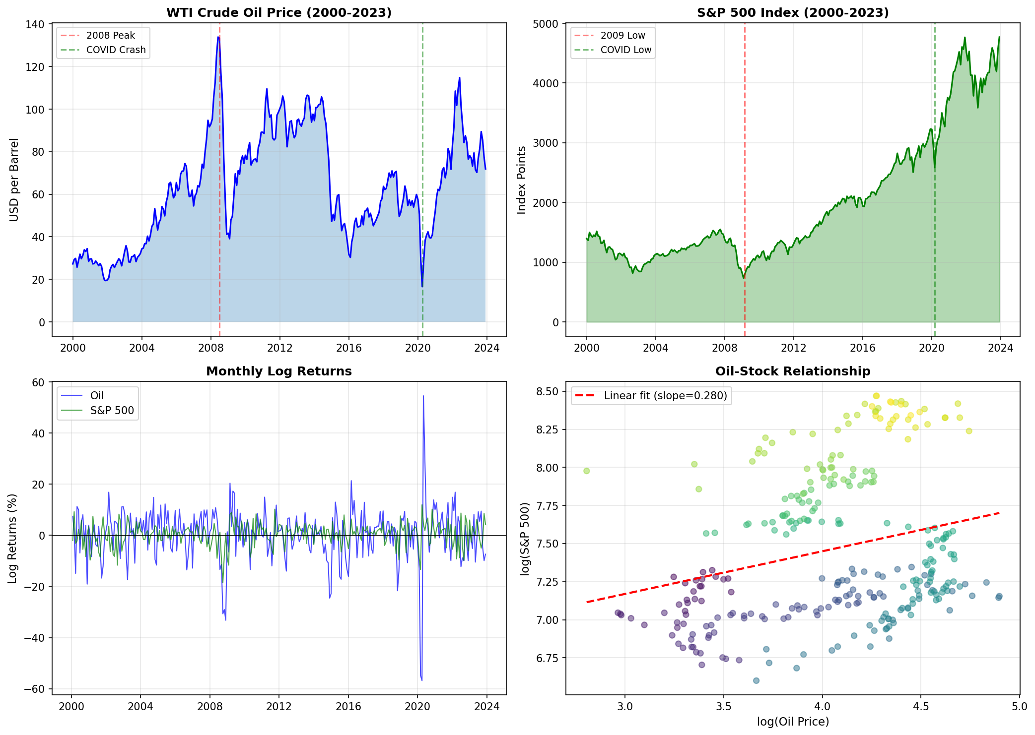
Figure 0: WTI Oil Prices and S&P 500 Index (2000-2023) with key events marked.
QARDL works best with I(1) variables that are cointegrated. Consider unit root testing before applying QARDL to ensure your variables satisfy the required assumptions.
Lag Selection
The pq_order() function selects optimal AR order (p) and distributed lag
order (q) using the Bayesian Information Criterion (BIC).
from qardl import pq_order

# Select optimal lag orders
p_opt, q_opt = pq_order(data, p_max=8, q_max=8)
print(f"Optimal AR order (p): {p_opt}")
print(f"Optimal DL order (q): {q_opt}")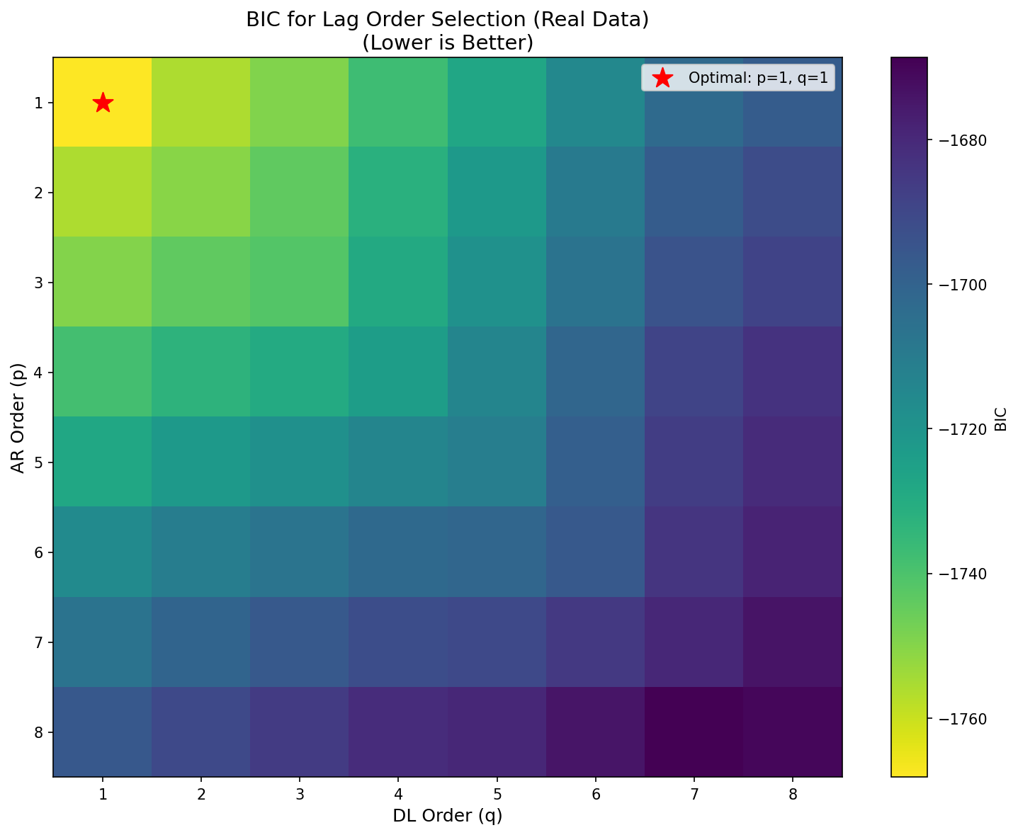
Figure 1: BIC values for different lag order combinations. The red star indicates the optimal (p, q) selection.
QARDL Estimation
The main estimation function qardl() estimates the Quantile ARDL model
for a given set of quantiles.
Model Specification
Estimation
from qardl import qardl

# Define quantiles
tau = np.array([0.10, 0.25, 0.50, 0.75, 0.90])

# Estimate QARDL model
qaOut = qardl(data, p=1, q=1, tau=tau)

# Print summary
print(qaOut.summary())
Output Structure
| Attribute | Description | Dimension |
|---|---|---|
bigbt |
Long-run parameters β | (k × s) × 1 |
bigbt_cov |
Covariance of β | (k × s) × (k × s) |
phi |
Short-run AR parameters φ | (p × s) × 1 |
phi_cov |
Covariance of φ | (p × s) × (p × s) |
gamma |
Short-run impact parameters γ | (k × s) × 1 |
gamma_cov |
Covariance of γ | (k × s) × (k × s) |
Where k = number of X variables, s = number of quantiles, p = AR order
Class-Based Interface
from qardl import QARDL

# Create model instance
model = QARDL(y=y, X=X, p=1, q=1, tau=[0.10, 0.25, 0.50, 0.75, 0.90])

# Fit model
results = model.fit()

# View summary
print(model.summary())
Parameter Interpretation
Long-run Parameters (β)
The long-run coefficient β(τ) measures the equilibrium relationship between y and x at quantile τ. It is computed as:
A positive β indicates that increases in x are associated with higher values of y in the long run, with the magnitude depending on the quantile.
Short-run Parameters (γ)
The parameter γ(τ) = θ0(τ) represents the contemporaneous impact of changes in x on y at quantile τ. This captures the immediate effect before the system adjusts toward the long-run equilibrium.
AR Parameters (φ)
The AR coefficients φi(τ) capture the persistence in the dependent variable. Values close to 1 indicate high persistence (slow mean reversion), while values significantly below 1 suggest faster adjustment dynamics.
| Quantile (τ) | β (Long-run) | φ (AR) | γ (Short-run) |
|---|---|---|---|
| 0.10 | 5.30 | 0.9963 | 0.0195 |
| 0.25 | 3.56 | 0.9985 | 0.0053 |
| 0.50 | -64.32 | 1.0001 | 0.0050 |
| 0.75 | 1.56 | 1.0010 | -0.0015 |
| 0.90 | 20.09 | 1.0008 | -0.0157 |
Visualization
QARDL provides several plotting functions to visualize estimation results.
Main Results Plot
from qardl import plot_qardl

fig = plot_qardl(qaOut, title="QARDL Estimation Results")
plt.savefig("qardl_results.png")
plt.show()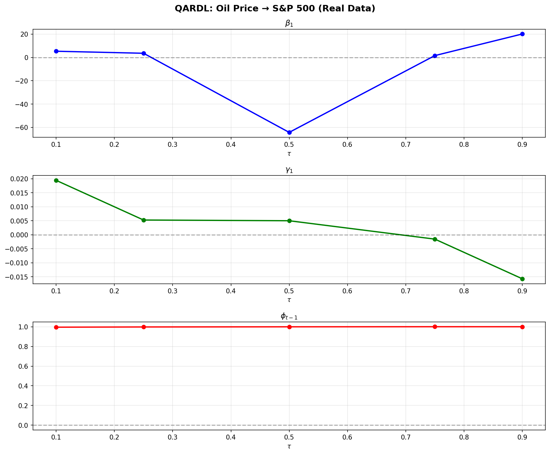
Figure 2: QARDL estimation results showing β, γ, and φ across quantiles.
Confidence Intervals
from qardl import plot_beta, plot_gamma, plot_phi

# Long-run parameters with 95% CI
fig = plot_beta(qaOut, with_ci=True, alpha=0.05)
plt.show()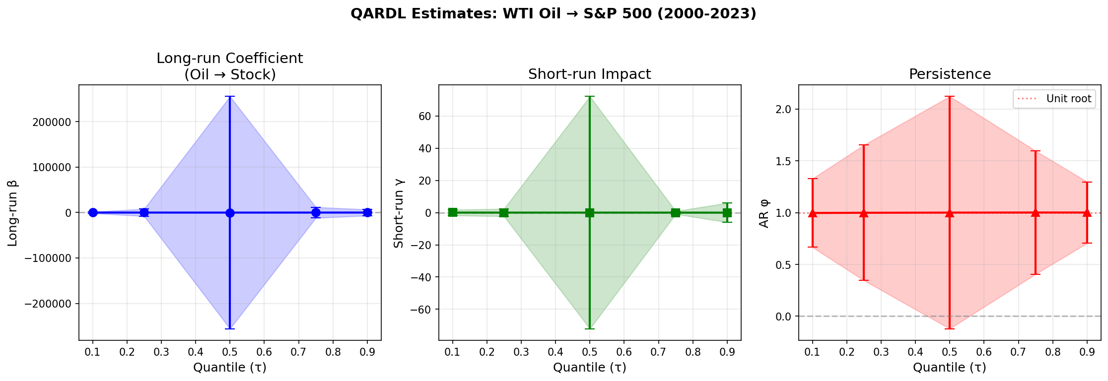
Figure 3: All QARDL coefficients with 95% confidence intervals across quantiles.
Wald Tests
QARDL provides Wald tests for testing hypotheses about parameter equality across quantiles and other restrictions.
Test Formulas
Long-run parameters: W = (n-1)² × (Rβ - r)' [R Σ R']⁻¹ (Rβ - r)
Short-run parameters: W = (n-1) × (Rθ - r)' [R Σ R']⁻¹ (Rθ - r)
Built-in Tests
from qardl import (
    test_long_run_equality,
    test_phi_equality,
    test_gamma_equality,
    test_cointegration
)

# Test long-run parameter equality across quantiles
wald_lr = test_long_run_equality(qaOut, data)
print(wald_lr.summary())

# Test AR parameter equality
wald_phi = test_phi_equality(qaOut, data)
print(wald_phi.summary())

# Test cointegration (β = 0)
wald_coint = test_cointegration(qaOut, data, param_index=0)
print(wald_coint.summary())Custom Wald Tests
from qardl import wtestlrb

# Test H0: β(τ=0.10) = β(τ=0.90)
k = qaOut.k
ss = len(tau)

# Create restriction matrix
R = np.zeros((1, k * ss))
R[0, 0] = 1     # β(τ=0.10)
R[0, k * (ss-1)] = -1  # β(τ=0.90)
r = np.zeros(1)

# Run test
wt, pv = wtestlrb(qaOut.bigbt, qaOut.bigbt_cov, R, r, data)
print(f"Wald statistic: {wt:.4f}")
print(f"P-value: {pv:.4f}")
Error Correction Model (ECM)
The ECM representation provides insights into the adjustment dynamics toward long-run equilibrium.
ECM Specification
Where ζ is the adjustment speed (should be negative for convergence), and the half-life of adjustment is -ln(2)/ζ.
from qardl import qardl_ecm, plot_ecm

# Estimate ECM
ecmOut = qardl_ecm(data, p=1, q=1, tau=tau)

# Print summary
print(ecmOut.summary())

# Get half-life for median quantile
hl = ecmOut.get_half_life(tau_idx=2)
print(f"Half-life at median: {hl:.2f} periods")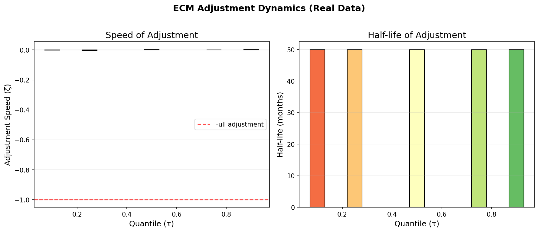
Figure 4: ECM adjustment speed and half-life across quantiles.
Rolling Window Estimation
Rolling QARDL estimation allows you to track parameter evolution over time, useful for detecting structural changes and time-varying relationships.
from qardl import rolling_qardl, create_wald_restrictions

# Create Wald test restrictions
tau_rolling = np.array([0.25, 0.50, 0.75])
wctl = create_wald_restrictions(k=1, p_max=8, num_tau=len(tau_rolling))

# Run rolling estimation
rqaOut = rolling_qardl(
    data,
    p_max=8,
    q_max=8,
    tau=tau_rolling,
    wctl=wctl,
    window_size=100
)

# Print summary
print(rqaOut.summary())

# Get specific estimates
beta_50 = rqaOut.get_beta(var_idx=0, tau_idx=1)  # β at τ=0.50
print(f"β(τ=0.50) mean: {np.mean(beta_50):.4f}")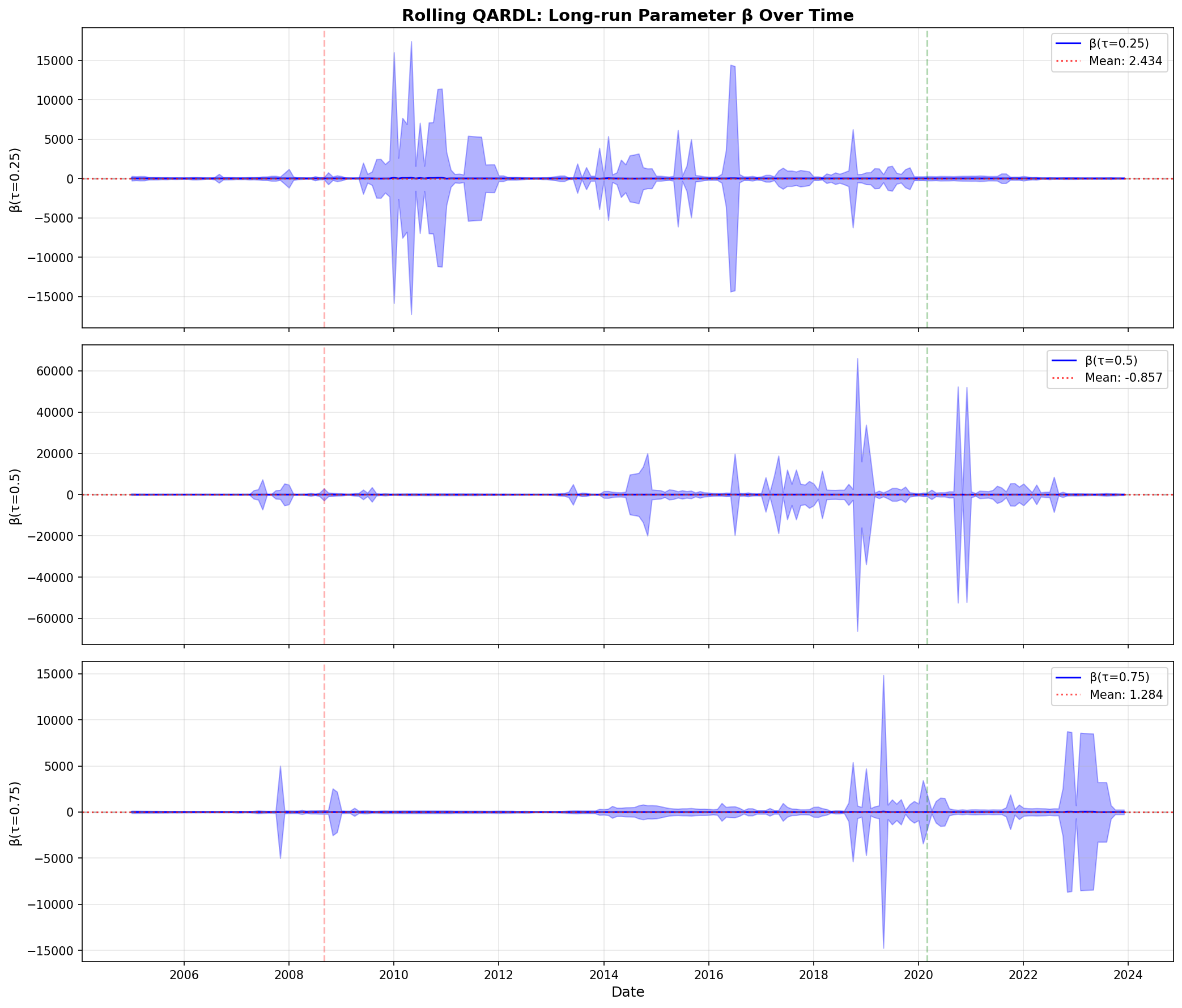
Figure 5: Rolling estimates of long-run parameter β with confidence bands.
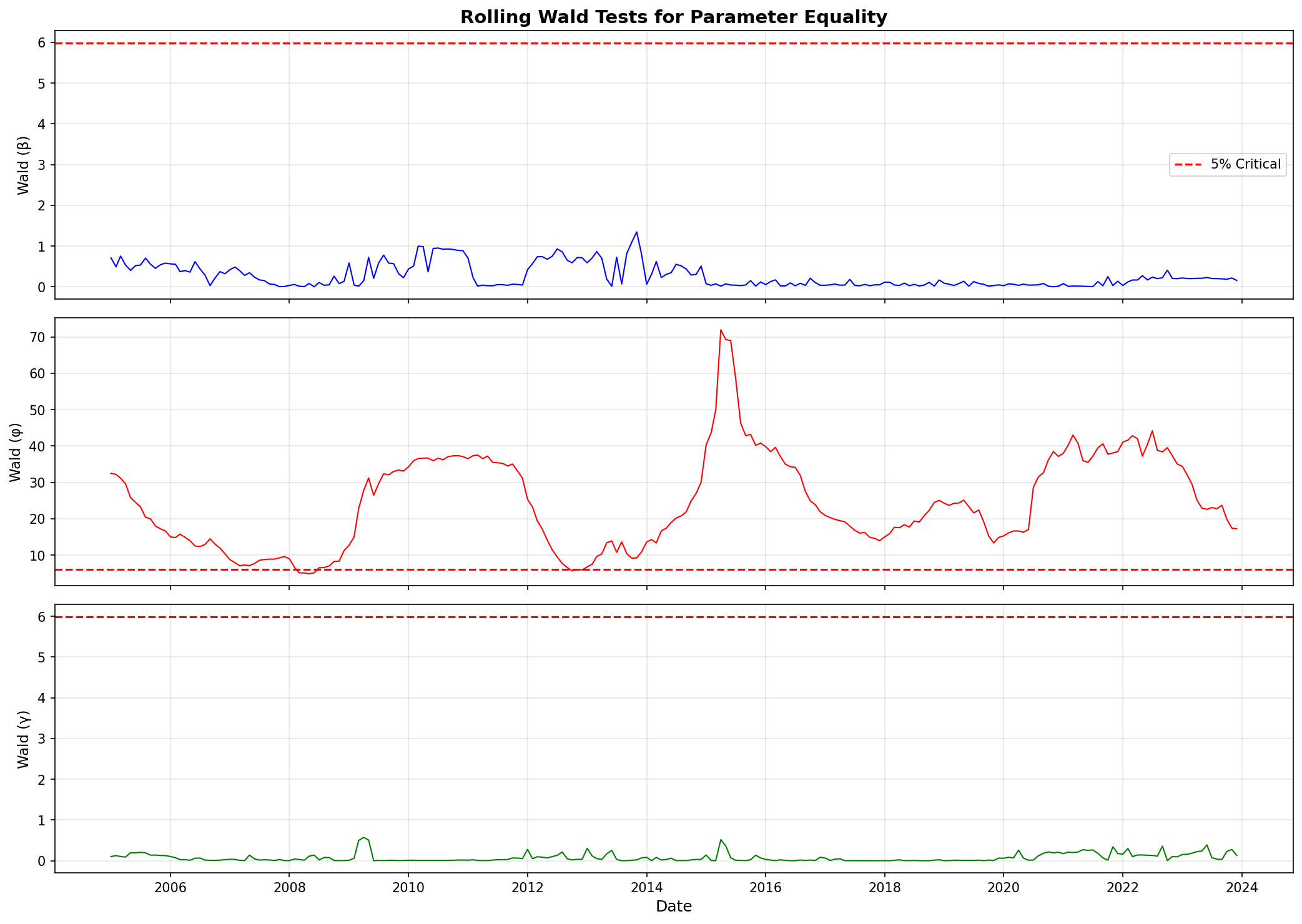
Figure 6: Rolling Wald test statistics for parameter equality.
Monte Carlo Simulation
QARDL includes tools for data generation and Monte Carlo simulation to validate the methodology and study finite-sample properties.
Data Generation
from qardl import qardl_ar2_sim, DGPParams

# Define DGP parameters
params = DGPParams(
    alpha=1.0,      # Intercept
    phi=0.5,        # AR coefficient
    theta0=2.0,     # Current X coefficient
    theta1=1.5,     # Lagged X coefficient
    rho=0.3         # X correlation
)

# True long-run coefficient
print(f"True β = γ/(1-φ) = {params.beta:.4f}")

# Generate data
y, X = qardl_ar2_sim(
    n=500,
    alpha=params.alpha,
    phi=params.phi,
    rho=params.rho,
    theta0=params.theta0,
    theta1=params.theta1,
    seed=42
)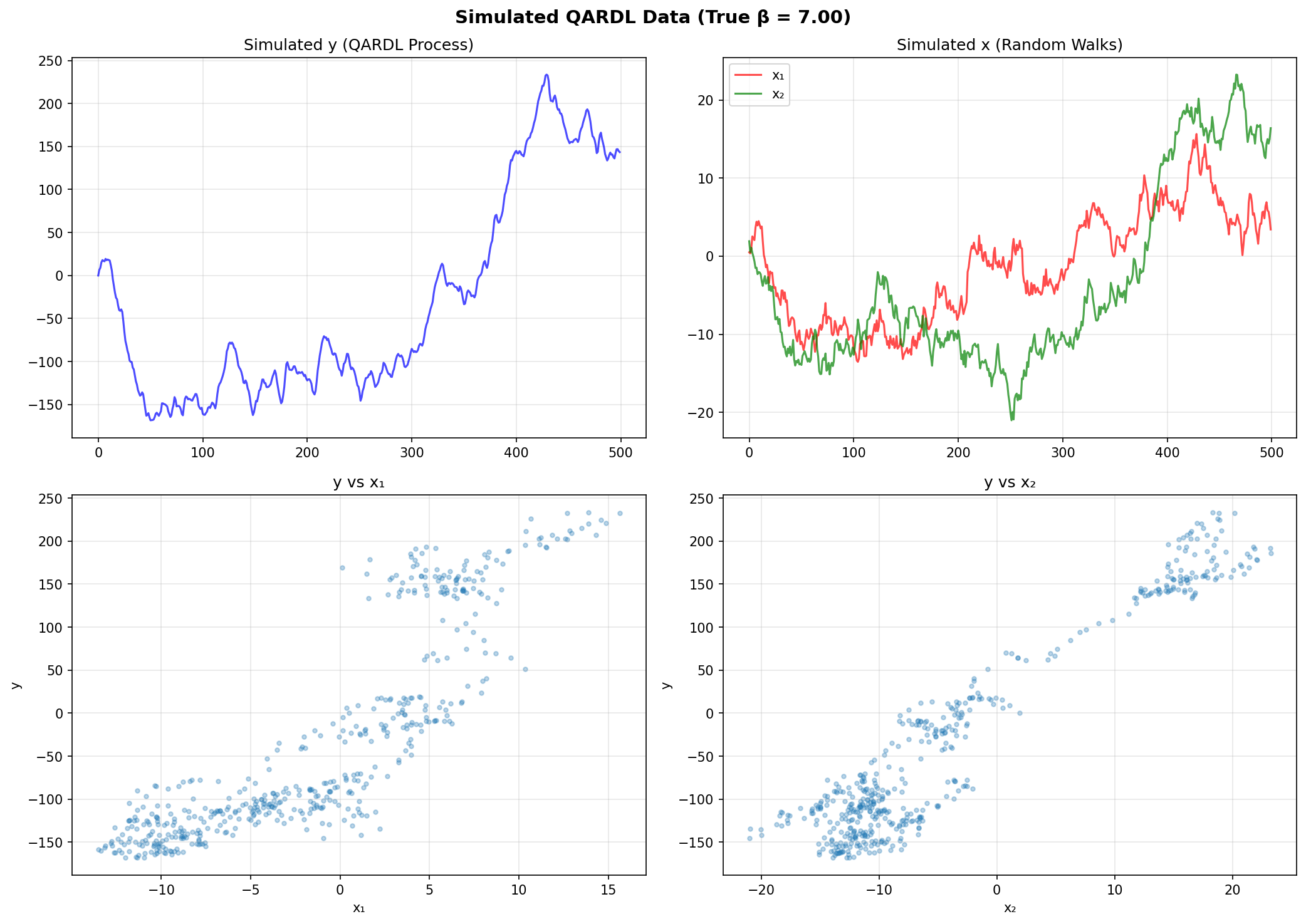
Figure 7: Simulated QARDL data with I(1) processes.
Monte Carlo Simulation
from qardl import simulate_wald_tests, print_simulation_results

# Run simulation
results = simulate_wald_tests(
    n=300,
    n_iter=1000,
    p=1,
    q=2,
    tau=np.array([0.25, 0.50, 0.75]),
    params=params,
    seed=42
)

# Print results
print_simulation_results(results)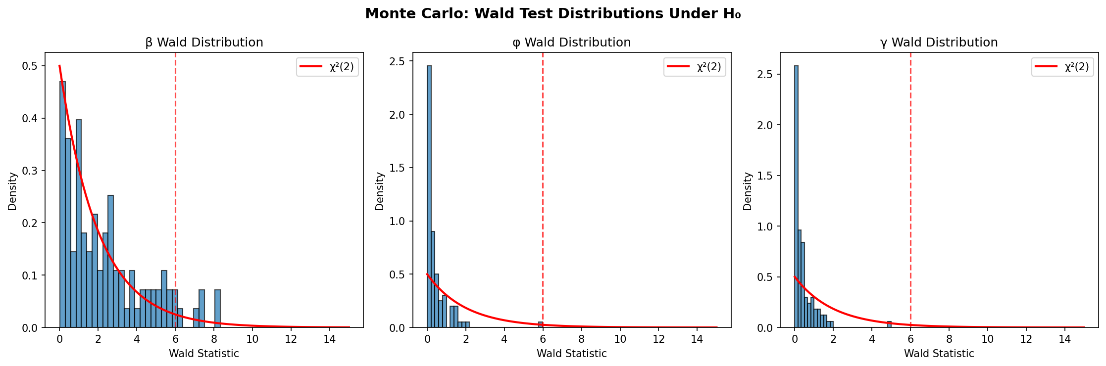
Figure 8: Distribution of Wald test statistics under H₀ compared to χ² distribution.
API Reference
Core Functions
| Function | Description | GAUSS Equivalent |
|---|---|---|
qardl(data, p, q, tau) |
Main QARDL estimation | qardl() |
QARDL class |
OOP interface for estimation | - |
pq_order(data, p_max, q_max) |
BIC lag selection | pqorder() |
Wald Tests
| Function | Description | GAUSS Equivalent |
|---|---|---|
wtestlrb() |
Long-run β test | wtestlrb.src |
wtestsrp() |
Short-run φ test | wtestsrp.src |
wtestsrg() |
Short-run γ test | wtestsrg.src |
ECM Functions
| Function | Description | MATLAB Equivalent |
|---|---|---|
qardl_ecm() |
ECM estimation | qardlecm.m |
convert_qardl_to_ecm() |
Convert QARDL to ECM params | - |
Plotting Functions
| Function | Description |
|---|---|
plot_qardl(qaOut) |
Plot all parameters |
plot_beta(qaOut, with_ci=True) |
Plot long-run with CI |
plot_gamma(qaOut, with_ci=True) |
Plot short-run γ |
plot_phi(qaOut, with_ci=True) |
Plot AR φ |
plot_rolling(rqaOut) |
Plot rolling results |
plot_ecm(ecmOut) |
Plot ECM results |
Theoretical Background
The QARDL Model
The Quantile Autoregressive Distributed Lag (QARDL) model extends the classical ARDL framework by allowing coefficients to vary across different quantiles of the conditional distribution. This enables the analysis of heterogeneous effects and asymmetric dynamics.
Model Formulation
The QARDL(p, q) model is specified as:
Long-run Equilibrium
The long-run coefficient is derived assuming the process reaches equilibrium where yt = yt-1 = ... = y* and xt = xt-1 = ... = x*:
Error Correction Form
The ECM representation allows analysis of adjustment dynamics:
The adjustment speed ζ(τ) = Σφi(τ) - 1 should be negative for convergence, with half-life = -ln(2)/ζ.
Inference
Wald tests are constructed using the asymptotic distribution of the quantile regression estimator with appropriate scaling factors:
- Long-run tests: Scale by (n-1)²
- Short-run tests: Scale by (n-1)
Citation
If you use this package in your research, please cite:
@article{cho2015quantile,
  title={Quantile cointegration in the autoregressive
         distributed-lag modeling framework},
  author={Cho, Jin Seo and Kim, Tae-hwan and Shin, Yongcheol},
  journal={Journal of Econometrics},
  volume={188},
  number={1},
  pages={281--300},
  year={2015},
  publisher={Elsevier}
}
Author
Dr. Merwan Roudane
Email: merwanroudane920@gmail.com
License
MIT License