tvccointreg — Time-Varying-Coefficient Regression & Generalized Cointegration

What it does

Conventional cointegration is inherently linear. Most economic relationships are not. This library closes that gap.

📈

Time-varying coefficients

Represent any nonlinear relationship as a model linear in variables with coefficients that drift over time (Swamy–Mehta / Granger theorem).

🧪

Generalized cointegration

Test whether the bias-free structural derivative is nonzero — a property of the real world, robust to nonlinearity and omitted variables.

🔬

Bias decomposition

Split every coefficient into bias-free, omitted-variable, and measurement-error parts via coefficient drivers.

∑

Standard inference

χ² / normal tests — not Dickey–Fuller — because inference rests on the stationary errors of the driver equations.

📊

Journal-ready output

Publication tables in text, LaTeX (booktabs) and HTML; Parula-themed plots out of the box.

🧩

One or many regressors

Each regressor gets its own time-varying coefficient and its own cointegration verdict.

A little theory

Based on Hall, S. G., Swamy, P. A. V. B. & Tavlas, G. S. (2015), A Note on Generalizing the Concept of Cointegration.

Any (possibly nonlinear) structural relationship $y_t=f_t(x_t,w_t)$ can be represented exactly as a model that is linear in variables but with time-varying coefficients:

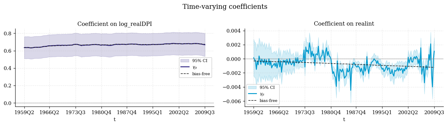
$$ y_t=\gamma_{0t}+\gamma_{1t}x_{1t}+\dots+\gamma_{K-1,t}x_{K-1,t} $$

Each coefficient is driven by observable coefficient drivers $z_{dt}$ plus a random error (Assumption 1):

$$ \gamma_{jt}=\pi_{j0}+\sum_{d}\pi_{jd}\,z_{dt}+\varepsilon_{jt} $$

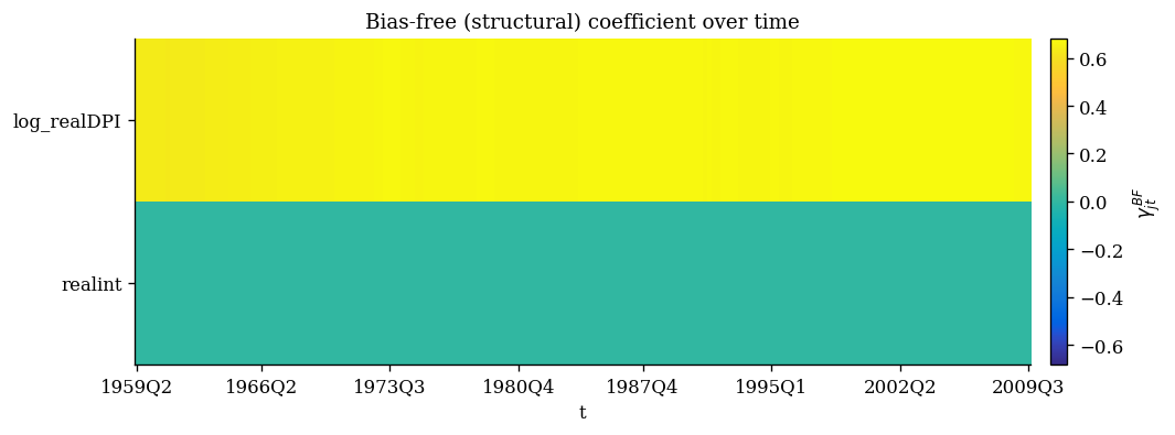
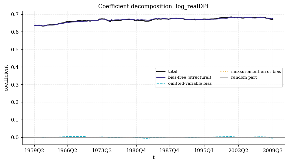
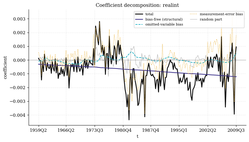
The drivers are split into three sets so the coefficient decomposes into a bias-free structural part plus omitted-variable and measurement-error biases. Two variables are generalized-cointegrated when — holding all other relevant preexisting conditions $w$ constant — the bias-free part of the derivative is nonzero:

$$ \frac{\partial y_t}{\partial x_t}\neq 0 \quad\Longleftrightarrow\quad \text{generalized cointegration.} $$

Substituting the driver equations into the model yields a concentrated linear model $y_t=w_t'\pi+u_t$ with a heteroskedastic but stationary error, estimated by iteratively rescaled GLS. Because the test statistic derives from the stationary driver-equation errors, inference is standard — no unit-root critical values.

Honest caveat. As in the paper, validity rests on choosing drivers that genuinely span the bias components (Assumption 1). This is an identifying assumption, not something the data can confirm — pick drivers plausibly correlated with the suspected misspecification.

Worked example — a US consumption function (real data)

Real US quarterly data (statsmodels macrodata, 1959Q1–2009Q3, 202 obs). Two structural regressors: disposable income and the real interest rate.

import numpy as np, pandas as pd
from statsmodels.datasets import macrodata
from tvccointreg import TVCModel, DriverSpec

d = macrodata.load_pandas().data
d.index = pd.period_range("1959Q1", periods=len(d), freq="Q")
z = lambda s:(s - s.mean())/s.std(ddof=0)

y = np.log(d["realcons"]).rename("log_realCons")   # log real consumption
X = pd.concat([np.log(d["realdpi"]).rename("log_realDPI"),
               d["realint"].rename("realint")], axis=1)
drivers = pd.DataFrame({
    "inc_lag":  z(np.log(d["realdpi"]).shift(1)),
    "trend":    z(pd.Series(np.arange(len(d)), index=d.index)),
    "unemp":    z(d["unemp"]),
    "rate_lag": z(d["realint"].shift(1))})
df = pd.concat([y, X, drivers], axis=1).dropna()

spec = DriverSpec(names=list(drivers.columns),
                  bias_free=["inc_lag","trend"],   # true coefficient drift
                  omitted=["unemp"],               # omitted-variable bias
                  measurement=["rate_lag"])         # measurement / dynamics

res = TVCModel(df["log_realCons"], df[["log_realDPI","realint"]],
               df[spec.names], driver_spec=spec).fit()
print(res.summary())
res.coint_test()

0.9998R² (fit)

2 / 2regressors cointegrated

3.5e-09residual ADF p (stationary)

9IRGLS iterations

Generalized cointegration test

One row per regressor — each gets its own Wald test on the bias-free block.

Regressor	Bias-free coef	Std. err	t	Wald	df	p-value	Cointegrated?
log_realDPI (income)	0.6666 ***	0.0658	10.13	111.40	3	< 0.0001	✔ Yes
realint (real rate)	−0.0007 **	0.0003	−2.26	8.37	3	0.039	✔ Yes

*** p<0.01, ** p<0.05. Income elasticity is positive (~0.67); the real interest rate enters negatively (intertemporal substitution). Both are genuine structural relationships, not spurious correlations.

Results — figures

Time-varying coefficients with 95% bands and the bias-free path.

Bias-free coefficient heatmap — Bias-free (structural) coefficients across regressors and time.

Income coefficient decomposition — Income coefficient: bias-free / omitted / measurement / random.

Rate coefficient decomposition — Real-rate coefficient decomposition.

Model fit and residuals — Actual vs. fitted consumption and the stationary residuals.

Full runnable script: examples/consumption_multivariate.py.

Installation & quick start

Pure-Python; depends only on NumPy, SciPy, pandas and Matplotlib.

Install

pip install tvccointreg

# with the ADF stationarity diagnostic
pip install "tvccointreg[adf]"

Minimal example

from tvccointreg import TVCModel, DriverSpec
from tvccointreg.datasets import \
    simulate_nonlinear_cointegration

sim = simulate_nonlinear_cointegration(T=300, seed=1)
spec = DriverSpec(names=list(sim.drivers.columns),
                  bias_free=["x_lag"], omitted=["w"])
res = TVCModel(sim.y, sim.X, sim.drivers,
               driver_spec=spec).fit()
print(res.summary())
res.coint_test()

📦 PyPI page 📖 Full documentation (README)

Author

Dr Merwan Roudane

Econometrician · author of open-source statistical software for R and Python.

Time-series econometrics Nonlinear & nonstationary models Quantile methods Statistical computing

GitHub Email PyPI packages

How to cite

@software{roudane_tvccointreg,
  author = {Merwan Roudane},
  title  = {tvccointreg: Time-Varying-Coefficient Regression and
            Generalized Cointegration in Python},
  year   = {2026},
  url    = {https://github.com/merwanroudane/tvccointreg}
}